16 Data insights
16.1 Learning Objectives
Use summary functions to explore the structure and completeness of a dataset.
Create simple summaries and grouped summaries using
count(),group_by(), andsummarise().Calculate descriptive statistics (mean, SD) across groups.
Use
janitortools Firke (2024) to quickly tabulate and summarise categorical data.Recognise how grouping can change the interpretation of summaries and relationships
16.2 A first glimpse
When starting with a new dataset, we want to get an initial idea:
How many rows and columns are there?
What are the column names?
What types of data are in each column?
What are their possible values or ranges?
These answers are useful to know before jumping into wrangling and cleaning data.
There are several ways to return an overview of your data, ranging in how comprehensively you wish to summarise your data’s structure.
16.3 The data
Rows: 344
Columns: 19
$ study_name        <chr> "PAL0708", "PAL0708", "PAL0708", "PAL0708", "PAL0708…
$ sample_number     <dbl> 1, 2, 3, 4, 5, 6, 7, 8, 9, 10, 11, 12, 13, 14, 15, 1…
$ species           <chr> "Adelie", "Adelie", "Adelie", "Adelie", "Adelie", "A…
$ region            <chr> "Anvers", "Anvers", "Anvers", "Anvers", "Anvers", "A…
$ island            <chr> "Torgersen", "Torgersen", "Torgersen", "Torgersen", …
$ stage             <chr> "Adult, 1 Egg Stage", "Adult, 1 Egg Stage", "Adult, …
$ individual_id     <chr> "N1A1", "N1A2", "N2A1", "N2A2", "N3A1", "N3A2", "N4A…
$ clutch_completion <chr> "Yes", "Yes", "Yes", "Yes", "Yes", "Yes", "No", "No"…
$ date_egg          <date> 2007-11-11, 2007-11-11, 2007-11-16, 2007-11-16, 200…
$ culmen_length_mm  <dbl> 39.1, 39.5, 40.3, NA, 36.7, 39.3, 38.9, 39.2, 34.1, …
$ culmen_depth_mm   <dbl> 18.7, 17.4, 18.0, NA, 19.3, 20.6, 17.8, 19.6, 18.1, …
$ flipper_length_mm <dbl> 181, 186, 195, NA, 193, 190, 181, 195, 193, 190, 186…
$ body_mass_g       <dbl> 3750, 3800, 3250, NA, 3450, 3650, 3625, 4675, 3475, …
$ sex               <chr> "Male", "Female", "Female", NA, "Female", "Male", "F…
$ delta_15_n_o_oo   <dbl> NA, 8.94956, 8.36821, NA, 8.76651, 8.66496, 9.18718,…
$ delta_13_c_o_oo   <dbl> NA, -24.69454, -25.33302, NA, -25.32426, -25.29805, …
$ comments          <chr> "Not enough blood for isotopes.", NA, NA, "Adult not…
$ year              <dbl> 2007, 2007, 2007, 2007, 2007, 2007, 2007, 2007, 2007…
$ mass_range <fct> mid penguin, mid penguin, smol penguin, NA, smol pen…tibble [344 × 19] (S3: tbl_df/tbl/data.frame)
$ study_name : chr [1:344] "PAL0708" "PAL0708" "PAL0708" "PAL0708" ...
$ sample_number : num [1:344] 1 2 3 4 5 6 7 8 9 10 ...
$ species : chr [1:344] "Adelie" "Adelie" "Adelie" "Adelie" ...
$ region : chr [1:344] "Anvers" "Anvers" "Anvers" "Anvers" ...
$ island : chr [1:344] "Torgersen" "Torgersen" "Torgersen" "Torgersen" ...
$ stage : chr [1:344] "Adult, 1 Egg Stage" "Adult, 1 Egg Stage" "Adult, 1 Egg Stage" "Adult, 1 Egg Stage" ...
$ individual_id : chr [1:344] "N1A1" "N1A2" "N2A1" "N2A2" ...
$ clutch_completion: chr [1:344] "Yes" "Yes" "Yes" "Yes" ...
$ date_egg : Date[1:344], format: "2007-11-11" "2007-11-11" ...
$ culmen_length_mm : num [1:344] 39.1 39.5 40.3 NA 36.7 39.3 38.9 39.2 34.1 42 ...
$ culmen_depth_mm : num [1:344] 18.7 17.4 18 NA 19.3 20.6 17.8 19.6 18.1 20.2 ...
$ flipper_length_mm: num [1:344] 181 186 195 NA 193 190 181 195 193 190 ...
$ body_mass_g : num [1:344] 3750 3800 3250 NA 3450 ...
$ sex : chr [1:344] "Male" "Female" "Female" NA ...
$ delta_15_n_o_oo : num [1:344] NA 8.95 8.37 NA 8.77 ...
$ delta_13_c_o_oo : num [1:344] NA -24.7 -25.3 NA -25.3 ...
$ comments : chr [1:344] "Not enough blood for isotopes." NA NA "Adult not sampled." ...
$ year : num [1:344] 2007 2007 2007 2007 2007 ...
$ mass_range : Factor w/ 3 levels "smol penguin",..: 2 2 1 NA 1 2 2 3 1 2 ...| Name | penguins |
| Number of rows | 344 |
| Number of columns | 19 |
| _______________________ | |
| Column type frequency: | |
| character | 9 |
| Date | 1 |
| factor | 1 |
| numeric | 8 |
| ________________________ | |
| Group variables | None |
Variable type: character
| skim_variable | n_missing | complete_rate | min | max | empty | n_unique | whitespace |
|---|---|---|---|---|---|---|---|
| study_name | 0 | 1.00 | 7 | 7 | 0 | 3 | 0 |
| species | 0 | 1.00 | 6 | 9 | 0 | 3 | 0 |
| region | 0 | 1.00 | 6 | 6 | 0 | 1 | 0 |
| island | 0 | 1.00 | 5 | 9 | 0 | 3 | 0 |
| stage | 0 | 1.00 | 18 | 18 | 0 | 1 | 0 |
| individual_id | 0 | 1.00 | 4 | 6 | 0 | 190 | 0 |
| clutch_completion | 0 | 1.00 | 2 | 3 | 0 | 2 | 0 |
| sex | 11 | 0.97 | 4 | 6 | 0 | 2 | 0 |
| comments | 290 | 0.16 | 18 | 68 | 0 | 10 | 0 |
Variable type: Date
| skim_variable | n_missing | complete_rate | min | max | median | n_unique |
|---|---|---|---|---|---|---|
| date_egg | 0 | 1 | 2007-11-09 | 2009-12-01 | 2008-11-09 | 50 |
Variable type: factor
| skim_variable | n_missing | complete_rate | ordered | n_unique | top_counts |
|---|---|---|---|---|---|
| mass_range | 2 | 0.99 | FALSE | 3 | mid: 146, cho: 118, smo: 78 |
Variable type: numeric
| skim_variable | n_missing | complete_rate | mean | sd | p0 | p25 | p50 | p75 | p100 | hist |
|---|---|---|---|---|---|---|---|---|---|---|
| sample_number | 0 | 1.00 | 63.15 | 40.43 | 1.00 | 29.00 | 58.00 | 95.25 | 152.00 | ▇▇▆▅▃ |
| culmen_length_mm | 2 | 0.99 | 43.92 | 5.46 | 32.10 | 39.23 | 44.45 | 48.50 | 59.60 | ▃▇▇▆▁ |
| culmen_depth_mm | 2 | 0.99 | 17.15 | 1.97 | 13.10 | 15.60 | 17.30 | 18.70 | 21.50 | ▅▅▇▇▂ |
| flipper_length_mm | 2 | 0.99 | 200.92 | 14.06 | 172.00 | 190.00 | 197.00 | 213.00 | 231.00 | ▂▇▃▅▂ |
| body_mass_g | 2 | 0.99 | 4201.75 | 801.95 | 2700.00 | 3550.00 | 4050.00 | 4750.00 | 6300.00 | ▃▇▆▃▂ |
| delta_15_n_o_oo | 14 | 0.96 | 8.73 | 0.55 | 7.63 | 8.30 | 8.65 | 9.17 | 10.03 | ▃▇▆▅▂ |
| delta_13_c_o_oo | 13 | 0.96 | -25.69 | 0.79 | -27.02 | -26.32 | -25.83 | -25.06 | -23.79 | ▆▇▅▅▂ |
| year | 0 | 1.00 | 2008.03 | 0.82 | 2007.00 | 2007.00 | 2008.00 | 2009.00 | 2009.00 | ▇▁▇▁▇ |
At this early stage, it’s helpful to assess whether your dataset meets your expectations. Consider if the data appear as anticipated. Are the values in each column reasonable? Are there any noticeable gaps or errors that might need to be corrected, or that could potentially render the data unusable?
Your turn
The dataset has rows (including the headers) and 17 columns.
It also provides information on the type of data in each column
<chr>- means character or text data<dbl>- means numerical data
Q Based on our summary functions are any variables assigned to the wrong data type (should be character when numeric or vice versa)?
Although some columns like date might not be correctly treated as character variables, they are not strictly numeric either, all other columns appear correct
Q Based on our summary functions do we have complete data for all variables?
No, they are 2 missing data points for body measurements (culmen, flipper, body mass), 11 missing data points for sex, 13/14 missing data points for blood isotopes (Delta N/C) and 290 missing data points for comments
We have just learned some ways to initially inspect our dataset. Keep in mind, we don’t expect everything to be perfect. This initial inspection is a good opportunity to identify where these issues might be and assess their severity.
When you are confident that the dataset is largely as expected, you are ready to start summarising your data.
16.4 Summary counts
In the previous section, we learned how to get an overview of our data’s structure, including the number of rows, the columns present, and any missing data. In this section, we will focus on summarising the data. Summarising data can provide insight into the scope and variation in our dataset, and help in evaluating its suitability for our analysis.
With our data we can count the total number of occurrences for different groups either by:
16.4.1 Filtering
16.4.2 Grouping
Or by grouping :
At this stage, these counts tell us what is in our dataset, not how variables relate to one another. To understand relationships, we will later need visualisations and models.
16.5 Frequency counts by subgroups
We can apply multiple grouping parameters at the same time - for example if we wish to know the frequency of observations by species and sex.
We can do this using dplyr or with functions in the janitor package:
Grouped summaries implicitly assume that differences between groups may matter. Later, we will see that ignoring important grouping variables can lead to misleading conclusions
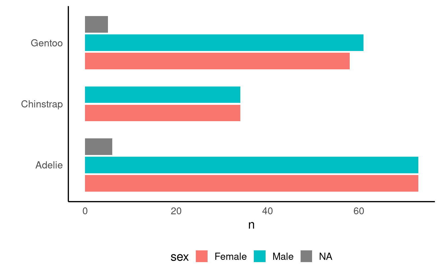
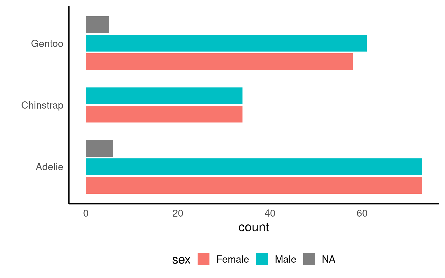
16.6 Visualising Frequencies
Graphs make summaries easier to interpret at a glance.
geom_col by default plots single values or “identity”, so numbers must be pre-calculated
penguins |>
  group_by(species,sex) |>
  count() |>
arrange(desc(n)) |>
ggplot(aes(x = species,
y = n,
fill = sex))+
geom_col(position=position_dodge2(preserve="single"))+
geom_label(aes(label = n),
position=position_dodge2(preserve="single",
width = .9))+ #<- dodge the text and label bars
coord_flip()+
labs(x = "")+
theme(legend.position = "bottom")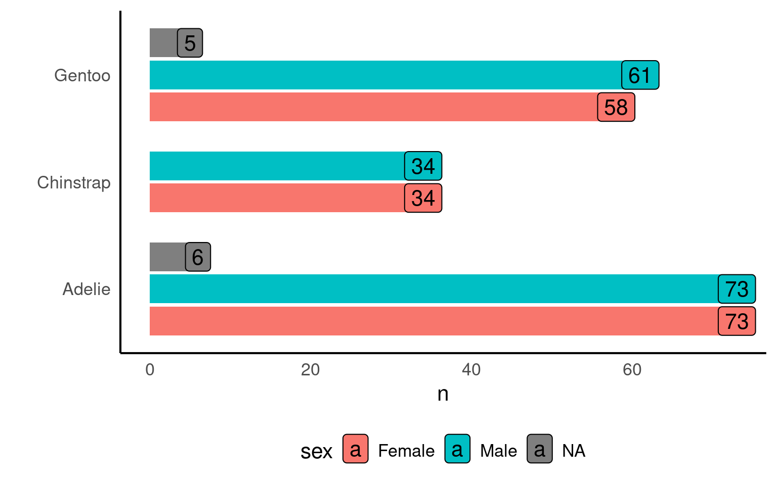
16.7 Exploring relationships between two variables
So far, we have focused on understanding the structure of the dataset and summarising individual variables or groups of observations. In many analyses, however, we are interested in how two variables vary together.
Exploring relationships between variables is an important step before modelling. At this stage, our goal is not to explain or predict outcomes, but to identify patterns, assess whether variables appear related, and consider whether these relationships differ across meaningful groups.
Plots are particularly important here, as numerical summaries alone can obscure important structure in the data.
16.7.1 Scatterplots
When both variables of interest are numeric, a scatterplot is the most informative first tool. Scatterplots allow us to see how values of one variable change in relation to another and whether any patterns are present.
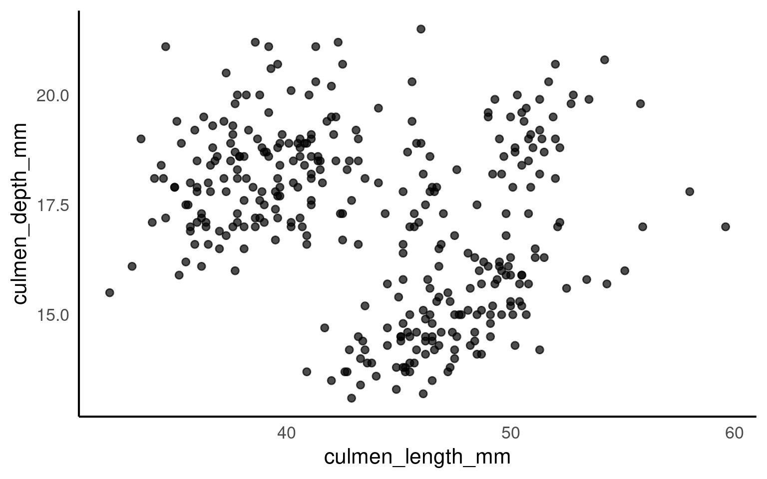
This plot shows the relationship between culmen length and culmen depth, with points coloured by penguin species.
Scatterplots such as this allow us to consider questions such as:
Do the variables appear positively or negatively associated?
Is the relationship approximately linear?
At this stage, we focus on visual comparison, rather than numerical summaries.
Your turn
Based on the scatterplot above, can you make a plot that includes species as an important grouping variable?
How does this change your observation?
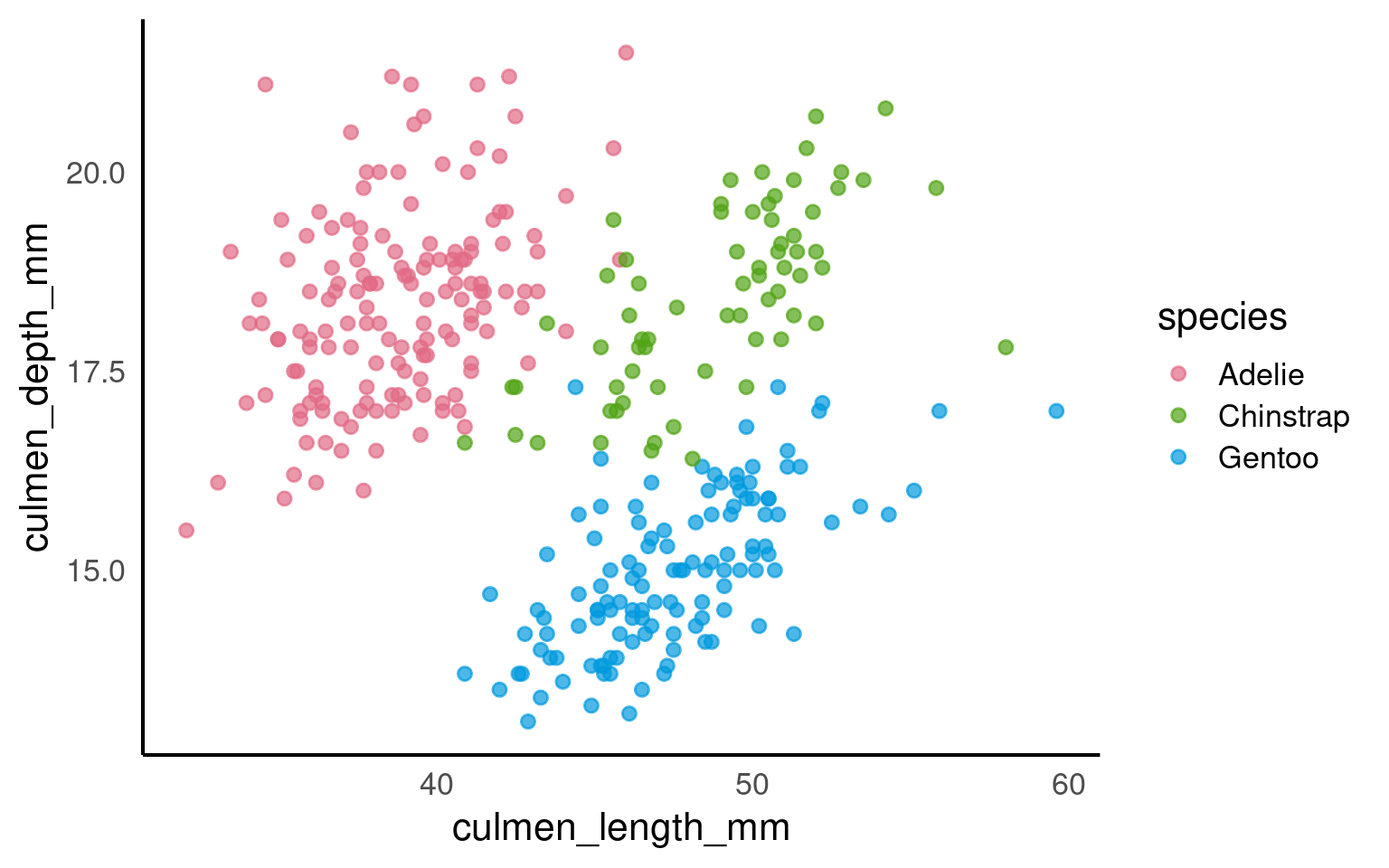
We now see a striking reversal of the apparent association between culmen length and depth, demonstrating the importance of considering groups in our analysis.
16.8 Correlation
In some situations, it can be useful to summarise the relationship between two numeric variables using a single numerical measure. Correlation provides such a summary by describing the strength and direction of a linear association between two variables.
Below, we calculate the overall correlation between culmen length and culmen depth across all observations.
| r |
|---|
| -0.2350529 |
Your turn
How can we generate summary statistics that reflect our important subgrouping (species)?
How does this change your observation?
16.9 Summary statistics
We can extend our summaries to show not just counts, but also measures of central tendency (mean) and spread (standard deviation).
These are powerful ways to understand variation within groups. These summaries describe average differences, but they do not tell us whether one variable predicts another, nor whether relationships differ across groups.
| species | mean_mass | sd_mass | n | median | iqr |
|---|---|---|---|---|---|
| Adelie | 3700.662 | 458.5661 | 152 | 3700 | 650.0 |
| Chinstrap | 3733.088 | 384.3351 | 68 | 3700 | 462.5 |
| Gentoo | 5076.016 | 504.1162 | 124 | 5000 | 800.0 |
Your turn
| species | sex | mean_mass_g | sd_mass_g | n |
|---|---|---|---|---|
| Adelie | Female | 3368.836 | 269.3801 | 73 |
| Adelie | Male | 4043.493 | 346.8116 | 73 |
| Chinstrap | Female | 3527.206 | 285.3339 | 34 |
| Chinstrap | Male | 3938.971 | 362.1376 | 34 |
| Gentoo | Female | 4679.741 | 281.5783 | 58 |
| Gentoo | Male | 5484.836 | 313.1586 | 61 |
16.9.1 Summarise multiple variables
These functions allow us to generate
summarise_at()
Summarise specific selected variables:
| species | flipper_length_mm | culmen_length_mm | culmen_depth_mm |
|---|---|---|---|
| Adelie | 189.9536 | 38.79139 | 18.34636 |
| Chinstrap | 195.8235 | 48.83382 | 18.42059 |
| Gentoo | 217.1870 | 47.50488 | 14.98211 |
summarise_if()
| species | sample_number | culmen_length_mm | culmen_depth_mm | flipper_length_mm | body_mass_g | delta_15_n_o_oo | delta_13_c_o_oo | year |
|---|---|---|---|---|---|---|---|---|
| Adelie | 76.5 | 38.79139 | 18.34636 | 189.9536 | 3700.662 | 8.859733 | -25.80419 | 2008.013 |
| Chinstrap | 34.5 | 48.83382 | 18.42059 | 195.8235 | 3733.088 | 9.356155 | -24.54654 | 2007.971 |
| Gentoo | 62.5 | 47.50488 | 14.98211 | 217.1870 | 5076.016 | 8.245338 | -26.18530 | 2008.081 |
16.10 Visualising distributions
Numerical summaries such as the mean and standard deviation provide useful information about a variable, but they do not show the full distribution of values.
Visualising distributions allows us to see how values are spread, whether observations are concentrated in particular ranges, and how distributions differ across groups.
Different plots are suited to different questions. In this section, we focus on choosing appropriate plots for comparing distributions across groups.
16.10.1 Boxplots for group comparisons
A boxplot provides a compact summary of the distribution of a numeric variable. It displays the median, the spread of the central values, and potential extreme observations, making it particularly useful for comparing distributions between groups.
Below, we visualise the distribution of body mass across penguin species.
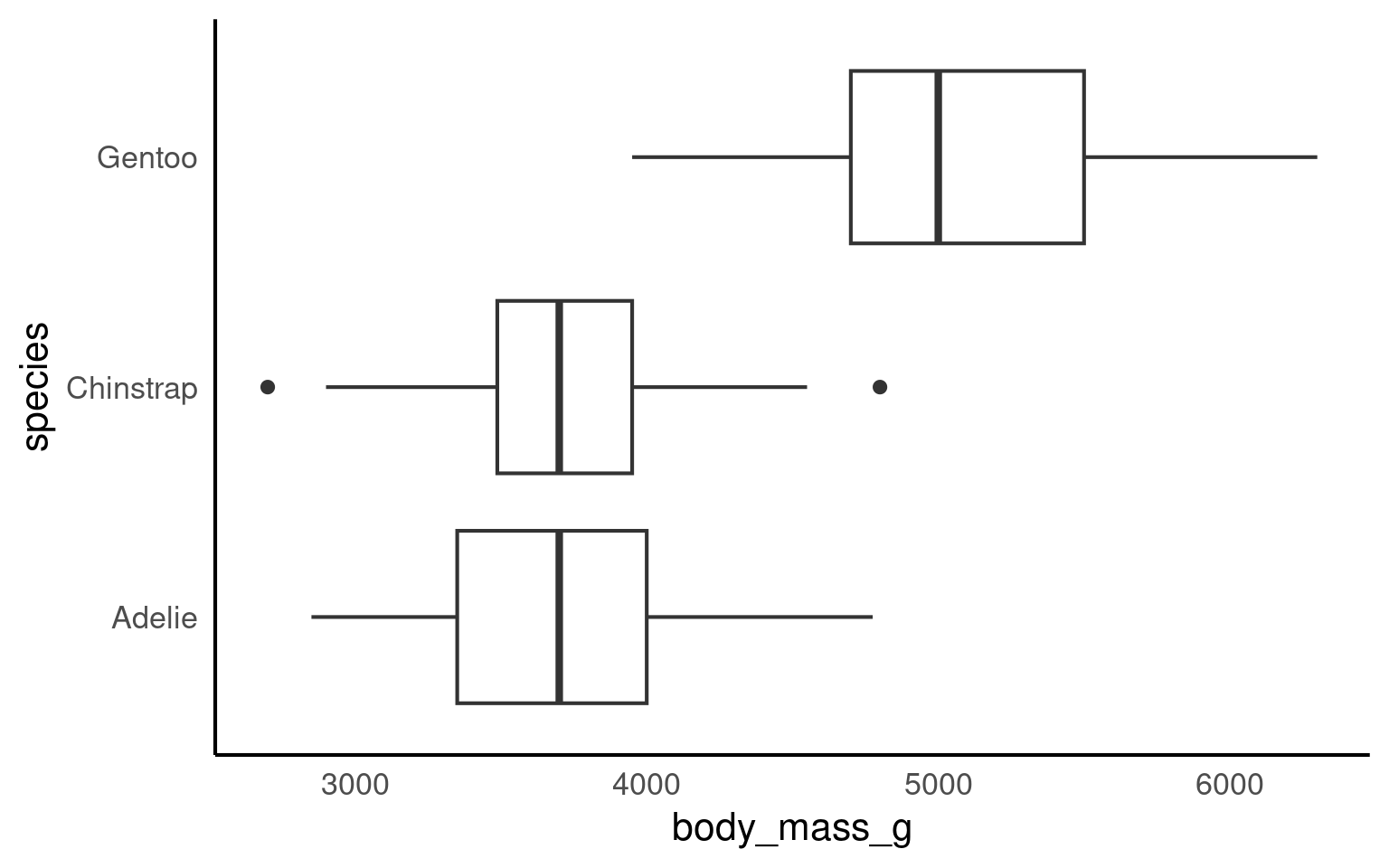
This plot allows us to compare:
Median body mass across species,
IQR (the interquartile range) the spread of values within each species,
Whether some species show more variability than others.
Boxplots are especially effective when the primary goal is comparison between groups, rather than detailed inspection of the distribution shape.
When visualising distributions, the choice of plot depends on the question being asked. In some cases, we are interested in comparing groups; in others, we want to explore the shape of the distribution within a single group.
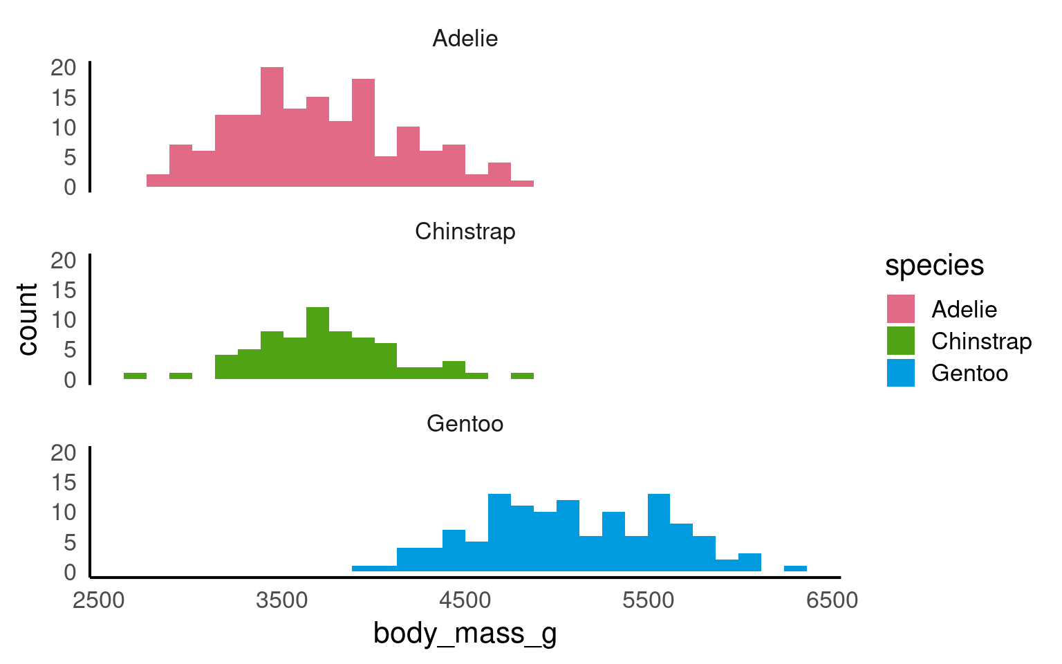
Your turn
You are exploring body mass in the penguin dataset.
If you wanted to explore the shape of the body-mass distribution for each single species, how would you change the plot? (Hint: consider changing the geom rather than the data.)
A histogram could be used by changing the geom to geom_histogram() and focusing on one species, as this allows closer inspection of the distribution shape within that group.
16.11 Useful summary functions
16.11.0.1 Measure of location:
mean(x): sum of x divided by the lengthmedian(x): 50% of x is above and 50% is below
16.11.0.2 Measure of variation:
sd(x): standard deviationIQR(x): interquartile range (robust equivalent of sd when outliers are present in the data)
16.11.0.3 Measure of rank:
min(x): minimum value of xmax(x): maximum value of xquantile(x, 0.25): 25% of x is below this value
16.11.0.4 Counts:
n(x): the number of element in xsum(!is.na(x)): count non-missing valuesn_distinct(x): count the number of unique value
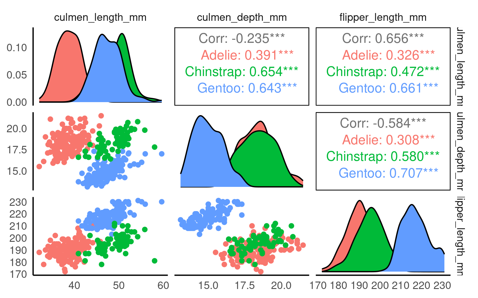
16.12 GGally
GGally is an invaluable tool in a researcher’s toolkit. It seamlessly extends the capabilities of the widely used ggplot2 package. With GGally, you can effortlessly create a variety of visualizations to explore and understand distributions and correlations among your variables. Its flexibility and ease of use make it a go-to choice for streamlining the process of creating insightful plots and charts for data analysis.
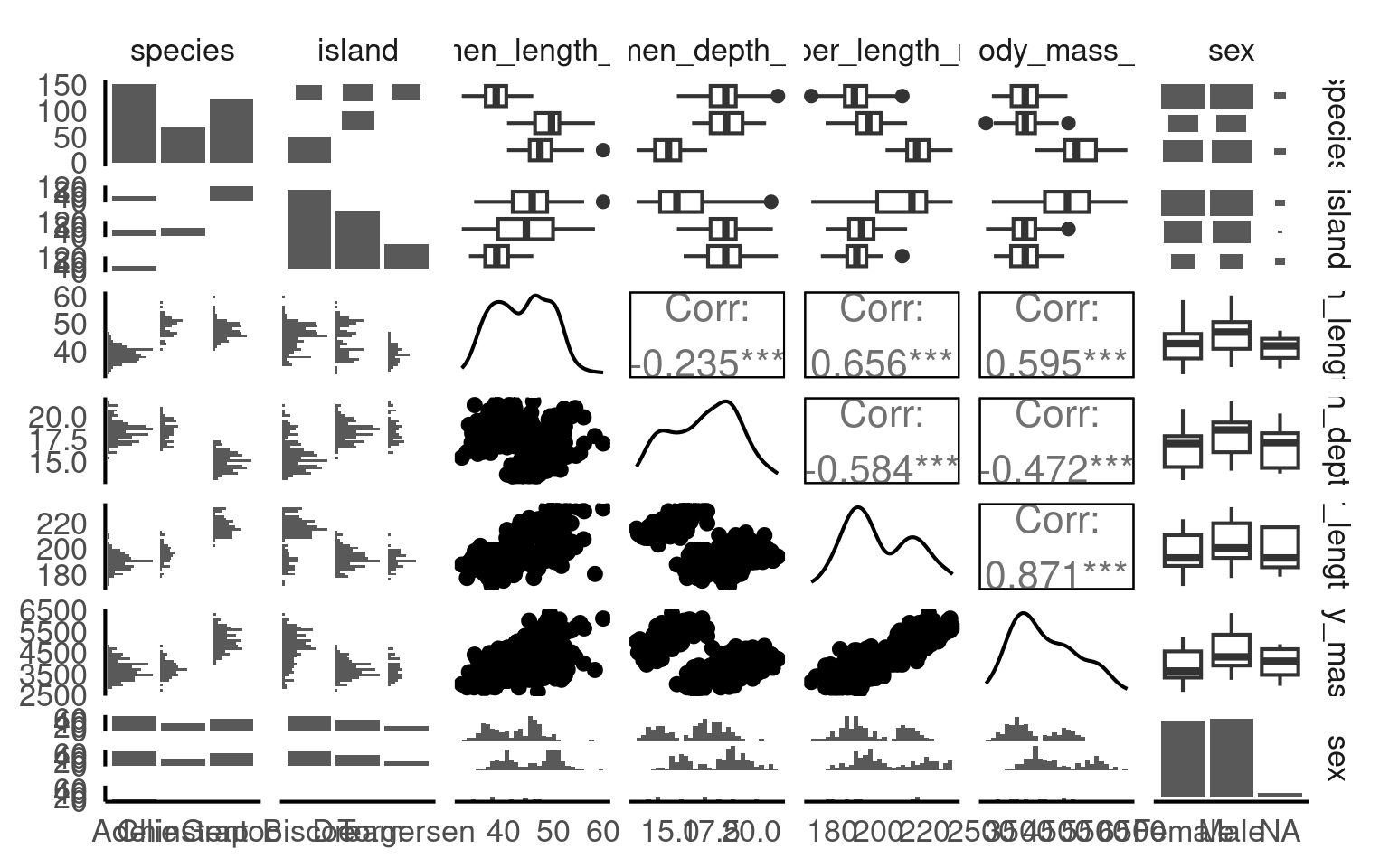
If we want to focus our exploration or include important grouping variables then this is also supported.
16.13 Summary
In this section we learned to:
-
Inspect structure and completeness
Use
glimpse(),str(), andskim()to understand column types, missing data, and variable ranges.Confirm that variables are stored in appropriate formats (e.g. numeric vs character).
-
Summarise counts and categories
Count observations using
count()andgroup_by()to explore dataset composition.Use
janitor::tabyl()for fast, readable cross-tabulations and percentages. -
Calculate descriptive statistics
- Compute group-wise summaries with
summarise()such as means, SDs, and counts.
- Compute group-wise summaries with
-
Visualise descriptive ranges and associations
- Use ggplot to produce a range of descriptive plots