24 Complex models
In the previous chapter Chapter 23 we worked through the process of including/excluding variables based on our causal hypotheses. However, we did not consider the potential role of complex interactions and in this chapter we will work through potential complexity in non-factorial experimental designs.
24.1 Experimental Design
In order to make clear hypothesis statements, and then test these - we need to have a good understanding of the experimental design
Your turn
Write some quick code to understand the distribution of treatment types and partner numbers across the experimental design.
Is the experiment a full factorialEvery possible combination of levels for multiple factors is present, providing a complete understanding of individual factor effects and their interactions design?
The experimental design is
Not all type x partner combinations exist:
Partners = 0 exists only for Control
Partners = 1,8 exist only for Virgin and Inseminated
This doesn’t affect our initial consideration of model structure, but we will revisit this later
24.2 Complex model interactions
Sometimes, the relationship between a covariate and the outcome differs between groups.
We have previously investigated models to examine the causal effect of mating types on male longevity - with five experimental groups
Control: Unmated flies (0 partners)
Virgin - 1 partner: Males paired with a single unmated female
Virgin - 8 partners: Males paired with multiple unmated females
Inseminated - 1 partner: Males paired with a single previously mated female
Inseminated - 8 partners: Males paired with multiple mated females
We now wish to consider some key questions in our experiment around interactions.
Does the number of females a male is paired with change the effect mating type has on male longevity?
Does the size of a male change the effect of mating type on male longevity?
| partners | type | n |
|---|---|---|
| 0 | Control | 25 |
| 1 | Inseminated | 25 |
| 1 | Virgin | 25 |
| 8 | Inseminated | 25 |
| 8 | Virgin | 25 |
This is a non-factorial design - not all type × partner combinations exist. Control flies only appear at 0 partners, while Virgin and Inseminated flies only appear at 1 or 8 partners.
Let’s start by fitting an interaction term with what seems like the obvious model:
\[ \text{longevity}_i = \beta_0 + \beta_1 \, \text{type}_i + \beta_2 \, \text{thorax}_i + \beta_3 \, \text{partners}_i + \beta_4 \, (\text{type}_i \times \text{thorax}_i) + \beta_5 \, (\text{type}_i \times \text{partners}_i) \varepsilon_i \]
This allows the the effect of size on longevity to depend on mating partner.
As a second interaction test it allows the effect of mating partner on longevity to depend on the number of partners
Before fitting new models, we should make sure our data is in the appropriate format:
Question 1. Why is it important for partners to be treated as a factor (rather than numeric)?
Partners is a numeric column - but this does not make sense with our experimental design, there are only three treatments with respect to number of partners, 0,1 or 8. If we leave partners as a numeric in our model, R will attempt to fit a single slope to explain the variance explained by partners as though it is a continuous variable. We have no reason to think the effect of partners is strictly linear, and with only three different observations it makes much more sense to treat this as categorical.
Your turn
Write a linear model that includes type, thorax and partners as main effects and include expressions to include an interaction effect between type:thorax and type:partners.
24.3 Issues with interpreting the fitted model
Let’s take a look at the fitted model now we have included our interaction terms:
Call:
lm(formula = longevity ~ type + thorax + partners + type:thorax +
    type:partners, data = dros_clean2)

Residuals:
     Min       1Q   Median       3Q      Max
-26.4634  -6.5711  -0.9363   6.8499  30.1715

Coefficients: (4 not defined because of singularities)
                          Estimate Std. Error t value Pr(>|t|)
(Intercept)               -50.2420    21.5582  -2.331  0.02149 *
typeInseminated             0.1163    27.0616   0.004  0.99658
typeVirgin                -15.3390    27.1769  -0.564  0.57355
thorax                    136.1268    25.6625   5.304 5.42e-07 ***
partners1                  13.1379     3.0940   4.246 4.38e-05 ***
partners8                       NA         NA      NA       NA
typeInseminated:thorax      4.7442    32.6180   0.145  0.88461
typeVirgin:thorax          -5.7505    32.8543  -0.175  0.86136
typeInseminated:partners1 -14.5153     4.3258  -3.356  0.00107 **
typeVirgin:partners1            NA         NA      NA       NA
typeInseminated:partners8       NA         NA      NA       NA
typeVirgin:partners8            NA         NA      NA       NA
---
Signif. codes:  0 '***' 0.001 '**' 0.01 '*' 0.05 '.' 0.1 ' ' 1

Residual standard error: 10.59 on 117 degrees of freedom
Multiple R-squared:  0.6568,    Adjusted R-squared:  0.6362
F-statistic: 31.98 on 7 and 117 DF,  p-value: < 2.2e-16
The intercept is Control at partners=0 (the reference levels for both factors). But look at what the other parameters mean:
- typeInseminated = -0.116: Difference between Inseminated and Control at partners=0
Problem: Inseminated flies don’t exist at partners=0! This is meaningless.
- partners1 = 13.14: Effect of having 1 partner for Control flies
Problem: Control flies don’t exist at partners=1! This is also meaningless.
Many NA values: R can’t estimate these parameters because the combinations don’t exist
While the model is technically functional - interpretation and coefficients are suboptimal. The Control level only exists at partners = 0, this creates a fundamental mismatch when trying to estimate values
Your turn
We need to revisit our key hypotheses and fix our model accordingly.
Can you write out specific testable questions we might have about interaction effects in our data?
Question 1: Within Virgin flies, does having 1 vs 8 partners affect longevity?
Question 2: Within Inseminated flies, does having 1 vs 8 partners affect longevity?
Question 3: At the same partner level, do Inseminated and Virgin flies differ in longevity?
Question 4: How do our mated treatments compare to unmated Controls?
Question 5: At the same body size, do Inseminated and Virgin flies differ in longevity?
With these questions in place we can “relevel” our factors to set the intercept to a different value - allowing for better comparisons
# By setting Virgin and partners = 1 as the first level in the factors for type and partners this will become the new intercept

dros_clean3 <- dros_clean2 |>
  mutate(type = fct_relevel(type, "Virgin"),
         partners = fct_relevel(partners, "1"))

# Refit the model

flyls3 <- lm(longevity ~ type +
               thorax +
               partners +
               type:thorax + # specifies the interaction effect
               type:partners, # specifies the interaction effect
             data = dros_clean3)

summary(flyls3)
Call:
lm(formula = longevity ~ type + thorax + partners + type:thorax +
    type:partners, data = dros_clean3)

Residuals:
     Min       1Q   Median       3Q      Max
-26.4634  -6.5711  -0.9363   6.8499  30.1715

Coefficients: (4 not defined because of singularities)
                          Estimate Std. Error t value Pr(>|t|)
(Intercept)                -52.443     17.313  -3.029  0.00302 **
typeControl                  2.201     27.649   0.080  0.93668
typeInseminated              0.940     24.094   0.039  0.96895
thorax                     130.376     20.514   6.355 4.15e-09 ***
partners0                       NA         NA      NA       NA
partners8                  -13.138      3.094  -4.246 4.38e-05 ***
typeControl:thorax           5.750     32.854   0.175  0.86136
typeInseminated:thorax      10.495     28.744   0.365  0.71569
typeControl:partners0           NA         NA      NA       NA
typeInseminated:partners0       NA         NA      NA       NA
typeControl:partners8           NA         NA      NA       NA
typeInseminated:partners8   14.515      4.326   3.356  0.00107 **
---
Signif. codes:  0 '***' 0.001 '**' 0.01 '*' 0.05 '.' 0.1 ' ' 1

Residual standard error: 10.59 on 117 degrees of freedom
Multiple R-squared:  0.6568,    Adjusted R-squared:  0.6362
F-statistic: 31.98 on 7 and 117 DF,  p-value: < 2.2e-16
The intercept is Virgin at partners=1 (the reference levels for both factors).
typeControl = 2.2 Difference between Virgin and Control (note control only has 0 partners)
typeInseminated = 0.940 Difference between Inseminated and Virgin at partners=1
Correct: Both treatments have examples of 1 partner.
- partners8 = -13.14 Difference between Virgin flies with 8 partners compare to 1
Correct
- Inseminated:partners8 = 14.515 Adjustment needed for estimating the effect of partners in Inseminated flies
Correct: Total difference in partners8 between Inseminated1 and Inseminated8 = -13.1 + 14.5 = 1.4 Total difference in partners8 between Virgin8 and Inseminated8 = 0.9 + 13.1 + 14.5 = 28.5
NA values: R can’t estimate these parameters because the combinations don’t exist
24.4 Determining a minimally sufficient model
- A significant interaction means the relationship between body size and longevity, and parners and longevity is not the same across partner types.
R compares the nested models via a likelihood ratio test (LRT):
H₀: β₃ = 0 (no interaction; same slope for all partner types)
H₁: β₃ ≠ 0 (interaction; slopes differ)
If the p-value is small (typically < 0.05), the more complex model explains significantly more variation — implying the interaction is meaningful.
| Df | Sum of Sq | RSS | AIC | F value | Pr(>F) | |
|---|---|---|---|---|---|---|
| NA | NA | 13129.69 | 597.7897 | NA | NA | |
| type:thorax | 2 | 14.98103 | 13144.67 | 593.9322 | 0.0667487 | 0.9354658 |
| type:partners | 1 | 1263.55212 | 14393.24 | 607.2750 | 11.2596451 | 0.0010686 |
The drop1 function produces a series of LRT where a term is removed from the model and the difference in variance is compared to the maximal model with an F-test. A significant result indicates a statisticall significant reduction in variance explained.
What does this mean?: We can safely remove terms that are non-significant as not helping explain variance in our data.
24.4.1 Refitting to produce the most optimal model
Having determined that there is evidence for an interaction effect between type:partners but there is not evidence for an interaction between type:thorax we can refit our model:
Call:
lm(formula = longevity ~ type + thorax + partners + type:partners,
    data = dros_clean3)

Residuals:
    Min      1Q  Median      3Q     Max
-26.189  -6.599  -0.989   6.408  30.244

Coefficients: (4 not defined because of singularities)
                          Estimate Std. Error t value Pr(>|t|)
(Intercept)                -57.002     10.629  -5.363 4.08e-07 ***
typeControl                  7.017      2.973   2.361 0.019874 *
typeInseminated              9.670      2.976   3.249 0.001507 **
thorax                     135.819     12.439  10.919  < 2e-16 ***
partners0                       NA         NA      NA       NA
partners8                  -12.933      3.009  -4.298 3.55e-05 ***
typeControl:partners0           NA         NA      NA       NA
typeInseminated:partners0       NA         NA      NA       NA
typeControl:partners8           NA         NA      NA       NA
typeInseminated:partners8   14.210      4.210   3.375 0.000996 ***
---
Signif. codes:  0 '***' 0.001 '**' 0.01 '*' 0.05 '.' 0.1 ' ' 1

Residual standard error: 10.51 on 119 degrees of freedom
Multiple R-squared:  0.6564,    Adjusted R-squared:  0.6419
F-statistic: 45.46 on 5 and 119 DF,  p-value: < 2.2e-16
This is our best fitting model - and the one we should report
24.5 Pairwise comparisons
Using the emmeans package is a very easy way to produce the estimate mean values (rather than mean differences) for different categories emmeans.
 type        thorax partners emmean   SE  df lower.CL upper.CL
 Virgin       0.821 1          54.5 2.11 119     50.3     58.7
 Control      0.821 1        nonEst   NA  NA       NA       NA
 Inseminated  0.821 1          64.2 2.10 119     60.0     68.3
 Virgin       0.821 0        nonEst   NA  NA       NA       NA
 Control      0.821 0          61.5 2.11 119     57.3     65.7
 Inseminated  0.821 0        nonEst   NA  NA       NA       NA
 Virgin       0.821 8          41.6 2.12 119     37.4     45.8
 Control      0.821 8        nonEst   NA  NA       NA       NA
 Inseminated  0.821 8          65.4 2.11 119     61.3     69.6

Confidence level used: 0.95
If the term pairs() is included then it will also include post-hoc pairwise comparisons between all levels with a tukey test (adjustment for multiple comparisons), we can turn off p-value adjustments by including the argument adjust = "none".
 contrast
 Virgin thorax0.82096 partners1 - Control thorax0.82096 partners1
 Virgin thorax0.82096 partners1 - Inseminated thorax0.82096 partners1
 Virgin thorax0.82096 partners1 - Virgin thorax0.82096 partners0
 Virgin thorax0.82096 partners1 - Control thorax0.82096 partners0
 Virgin thorax0.82096 partners1 - Inseminated thorax0.82096 partners0
 Virgin thorax0.82096 partners1 - Virgin thorax0.82096 partners8
 Virgin thorax0.82096 partners1 - Control thorax0.82096 partners8
 Virgin thorax0.82096 partners1 - Inseminated thorax0.82096 partners8
 Control thorax0.82096 partners1 - Inseminated thorax0.82096 partners1
 Control thorax0.82096 partners1 - Virgin thorax0.82096 partners0
 Control thorax0.82096 partners1 - Control thorax0.82096 partners0
 Control thorax0.82096 partners1 - Inseminated thorax0.82096 partners0
 Control thorax0.82096 partners1 - Virgin thorax0.82096 partners8
 Control thorax0.82096 partners1 - Control thorax0.82096 partners8
 Control thorax0.82096 partners1 - Inseminated thorax0.82096 partners8
 Inseminated thorax0.82096 partners1 - Virgin thorax0.82096 partners0
 Inseminated thorax0.82096 partners1 - Control thorax0.82096 partners0
 Inseminated thorax0.82096 partners1 - Inseminated thorax0.82096 partners0
 Inseminated thorax0.82096 partners1 - Virgin thorax0.82096 partners8
 Inseminated thorax0.82096 partners1 - Control thorax0.82096 partners8
 Inseminated thorax0.82096 partners1 - Inseminated thorax0.82096 partners8
 Virgin thorax0.82096 partners0 - Control thorax0.82096 partners0
 Virgin thorax0.82096 partners0 - Inseminated thorax0.82096 partners0
 Virgin thorax0.82096 partners0 - Virgin thorax0.82096 partners8
 Virgin thorax0.82096 partners0 - Control thorax0.82096 partners8
 Virgin thorax0.82096 partners0 - Inseminated thorax0.82096 partners8
 Control thorax0.82096 partners0 - Inseminated thorax0.82096 partners0
 Control thorax0.82096 partners0 - Virgin thorax0.82096 partners8
 Control thorax0.82096 partners0 - Control thorax0.82096 partners8
 Control thorax0.82096 partners0 - Inseminated thorax0.82096 partners8
 Inseminated thorax0.82096 partners0 - Virgin thorax0.82096 partners8
 Inseminated thorax0.82096 partners0 - Control thorax0.82096 partners8
 Inseminated thorax0.82096 partners0 - Inseminated thorax0.82096 partners8
 Virgin thorax0.82096 partners8 - Control thorax0.82096 partners8
 Virgin thorax0.82096 partners8 - Inseminated thorax0.82096 partners8
 Control thorax0.82096 partners8 - Inseminated thorax0.82096 partners8
 estimate   SE  df t.ratio p.value
   nonEst   NA  NA      NA      NA
    -9.67 2.98 119  -3.249  0.0015
   nonEst   NA  NA      NA      NA
    -7.02 2.97 119  -2.361  0.0199
   nonEst   NA  NA      NA      NA
    12.93 3.01 119   4.298 <0.0001
   nonEst   NA  NA      NA      NA
   -10.95 3.00 119  -3.650  0.0004
   nonEst   NA  NA      NA      NA
   nonEst   NA  NA      NA      NA
   nonEst   NA  NA      NA      NA
   nonEst   NA  NA      NA      NA
   nonEst   NA  NA      NA      NA
   nonEst   NA  NA      NA      NA
   nonEst   NA  NA      NA      NA
   nonEst   NA  NA      NA      NA
     2.65 2.98 119   0.891  0.3745
   nonEst   NA  NA      NA      NA
    22.60 2.99 119   7.560 <0.0001
   nonEst   NA  NA      NA      NA
    -1.28 2.98 119  -0.428  0.6695
   nonEst   NA  NA      NA      NA
   nonEst   NA  NA      NA      NA
   nonEst   NA  NA      NA      NA
   nonEst   NA  NA      NA      NA
   nonEst   NA  NA      NA      NA
   nonEst   NA  NA      NA      NA
    19.95 3.01 119   6.636 <0.0001
   nonEst   NA  NA      NA      NA
    -3.93 3.00 119  -1.311  0.1923
   nonEst   NA  NA      NA      NA
   nonEst   NA  NA      NA      NA
   nonEst   NA  NA      NA      NA
   nonEst   NA  NA      NA      NA
   -23.88 2.97 119  -8.031 <0.0001
   nonEst   NA  NA      NA      NA
In this example a Tukey HSD test adjustment has been applied - the p-values have been adjusted for a family of 5 estimates representing the five different experimental groups
 contrast
 Virgin thorax0.82096 partners1 - Control thorax0.82096 partners1
 Virgin thorax0.82096 partners1 - Inseminated thorax0.82096 partners1
 Virgin thorax0.82096 partners1 - Virgin thorax0.82096 partners0
 Virgin thorax0.82096 partners1 - Control thorax0.82096 partners0
 Virgin thorax0.82096 partners1 - Inseminated thorax0.82096 partners0
 Virgin thorax0.82096 partners1 - Virgin thorax0.82096 partners8
 Virgin thorax0.82096 partners1 - Control thorax0.82096 partners8
 Virgin thorax0.82096 partners1 - Inseminated thorax0.82096 partners8
 Control thorax0.82096 partners1 - Inseminated thorax0.82096 partners1
 Control thorax0.82096 partners1 - Virgin thorax0.82096 partners0
 Control thorax0.82096 partners1 - Control thorax0.82096 partners0
 Control thorax0.82096 partners1 - Inseminated thorax0.82096 partners0
 Control thorax0.82096 partners1 - Virgin thorax0.82096 partners8
 Control thorax0.82096 partners1 - Control thorax0.82096 partners8
 Control thorax0.82096 partners1 - Inseminated thorax0.82096 partners8
 Inseminated thorax0.82096 partners1 - Virgin thorax0.82096 partners0
 Inseminated thorax0.82096 partners1 - Control thorax0.82096 partners0
 Inseminated thorax0.82096 partners1 - Inseminated thorax0.82096 partners0
 Inseminated thorax0.82096 partners1 - Virgin thorax0.82096 partners8
 Inseminated thorax0.82096 partners1 - Control thorax0.82096 partners8
 Inseminated thorax0.82096 partners1 - Inseminated thorax0.82096 partners8
 Virgin thorax0.82096 partners0 - Control thorax0.82096 partners0
 Virgin thorax0.82096 partners0 - Inseminated thorax0.82096 partners0
 Virgin thorax0.82096 partners0 - Virgin thorax0.82096 partners8
 Virgin thorax0.82096 partners0 - Control thorax0.82096 partners8
 Virgin thorax0.82096 partners0 - Inseminated thorax0.82096 partners8
 Control thorax0.82096 partners0 - Inseminated thorax0.82096 partners0
 Control thorax0.82096 partners0 - Virgin thorax0.82096 partners8
 Control thorax0.82096 partners0 - Control thorax0.82096 partners8
 Control thorax0.82096 partners0 - Inseminated thorax0.82096 partners8
 Inseminated thorax0.82096 partners0 - Virgin thorax0.82096 partners8
 Inseminated thorax0.82096 partners0 - Control thorax0.82096 partners8
 Inseminated thorax0.82096 partners0 - Inseminated thorax0.82096 partners8
 Virgin thorax0.82096 partners8 - Control thorax0.82096 partners8
 Virgin thorax0.82096 partners8 - Inseminated thorax0.82096 partners8
 Control thorax0.82096 partners8 - Inseminated thorax0.82096 partners8
 estimate   SE  df t.ratio p.value
   nonEst   NA  NA      NA      NA
    -9.67 2.98 119  -3.249  0.0129
   nonEst   NA  NA      NA      NA
    -7.02 2.97 119  -2.361  0.1336
   nonEst   NA  NA      NA      NA
    12.93 3.01 119   4.298  0.0003
   nonEst   NA  NA      NA      NA
   -10.95 3.00 119  -3.650  0.0035
   nonEst   NA  NA      NA      NA
   nonEst   NA  NA      NA      NA
   nonEst   NA  NA      NA      NA
   nonEst   NA  NA      NA      NA
   nonEst   NA  NA      NA      NA
   nonEst   NA  NA      NA      NA
   nonEst   NA  NA      NA      NA
   nonEst   NA  NA      NA      NA
     2.65 2.98 119   0.891  0.8996
   nonEst   NA  NA      NA      NA
    22.60 2.99 119   7.560 <0.0001
   nonEst   NA  NA      NA      NA
    -1.28 2.98 119  -0.428  0.9929
   nonEst   NA  NA      NA      NA
   nonEst   NA  NA      NA      NA
   nonEst   NA  NA      NA      NA
   nonEst   NA  NA      NA      NA
   nonEst   NA  NA      NA      NA
   nonEst   NA  NA      NA      NA
    19.95 3.01 119   6.636 <0.0001
   nonEst   NA  NA      NA      NA
    -3.93 3.00 119  -1.311  0.6849
   nonEst   NA  NA      NA      NA
   nonEst   NA  NA      NA      NA
   nonEst   NA  NA      NA      NA
   nonEst   NA  NA      NA      NA
   -23.88 2.97 119  -8.031 <0.0001
   nonEst   NA  NA      NA      NA

P value adjustment: tukey method for comparing a family of 5 estimates It depends - adjusted p-values are more conservative - and there is a good reason to use these (preventing Type 1 errors) - especially if we didn’t have a clear set of initial hypotheses. However, in this example we have a clear experimental design, and we aren’t actually interested in looking at every comparison possible. We are interested in the difference between the three treatment groups and whether partner number changes this. With these careful planned contrasts we should be ok using unadjusted p-values
24.6 Visualising models
We can make visualisations of our models with ggplot().
Because we have included thorax as a stabilising predictor in our models we have some options on how to present our results:
Thorax does not interact with other predictors - as such it is a constant and
emmeanshas set these to the mean value within the dataset, so comparisons are constant between categories at the average value of all continuous variables.If we wish to model continuous predictions we need to specify these by asking for model predictions across the observed range of thorax values
means |>
    as_tibble() |>
    ggplot(aes(x=type, y = emmean, colour = partners, fill = partners))+
    geom_pointrange(aes(ymin=lower.CL, ymax=upper.CL), position = position_dodge(width =.2))+
    geom_point(data = dros_clean3,
               aes(x = type,
                   y = longevity),
               show.legend = FALSE,
               alpha = .2,
               position = position_dodge(width =.2))+
  scale_colour_discrete_qualitative() +
  theme_classic()+
  theme(strip.text = element_blank())+
  facet_wrap(~factor(type,
                     levels = c("Control",
                                "Inseminated",
                                "Virgin")),
             scales = "free_x")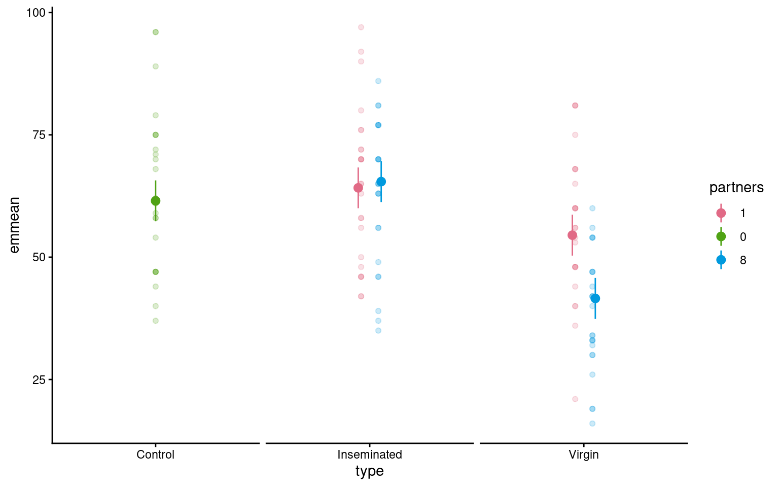
# use the final model to produce model predictions set to the new dataframe


emmeans::emmeans(flyls4,
                 specs = ~ type + thorax + partners,
                 at = list(thorax = seq(0.64,0.94, .1))) |>
  as_tibble() |>
  ggplot(
       aes(x=thorax,
           y = emmean,
           colour = type,
           fill = type))+
  geom_ribbon(aes(ymin=lower.CL,
                  ymax=upper.CL),
              alpha = 0.2)+
    geom_line(linetype = "dashed",
              show.legend = FALSE)+
  geom_point(data = dros_clean,
             aes(x = thorax,
                 y = longevity),
             show.legend = FALSE)+
scale_fill_discrete_qualitative() +
scale_colour_discrete_qualitative() +
  labs(y = "Lifespan in days",
       x = "Thorax length (mm)",
       fill = "Type of female exposure")+
  guides(colour = "none")+
  theme_classic()+
  theme(legend.position = "bottom")+
    facet_wrap(~factor(partners,
                       levels = c(0, 1, 8)))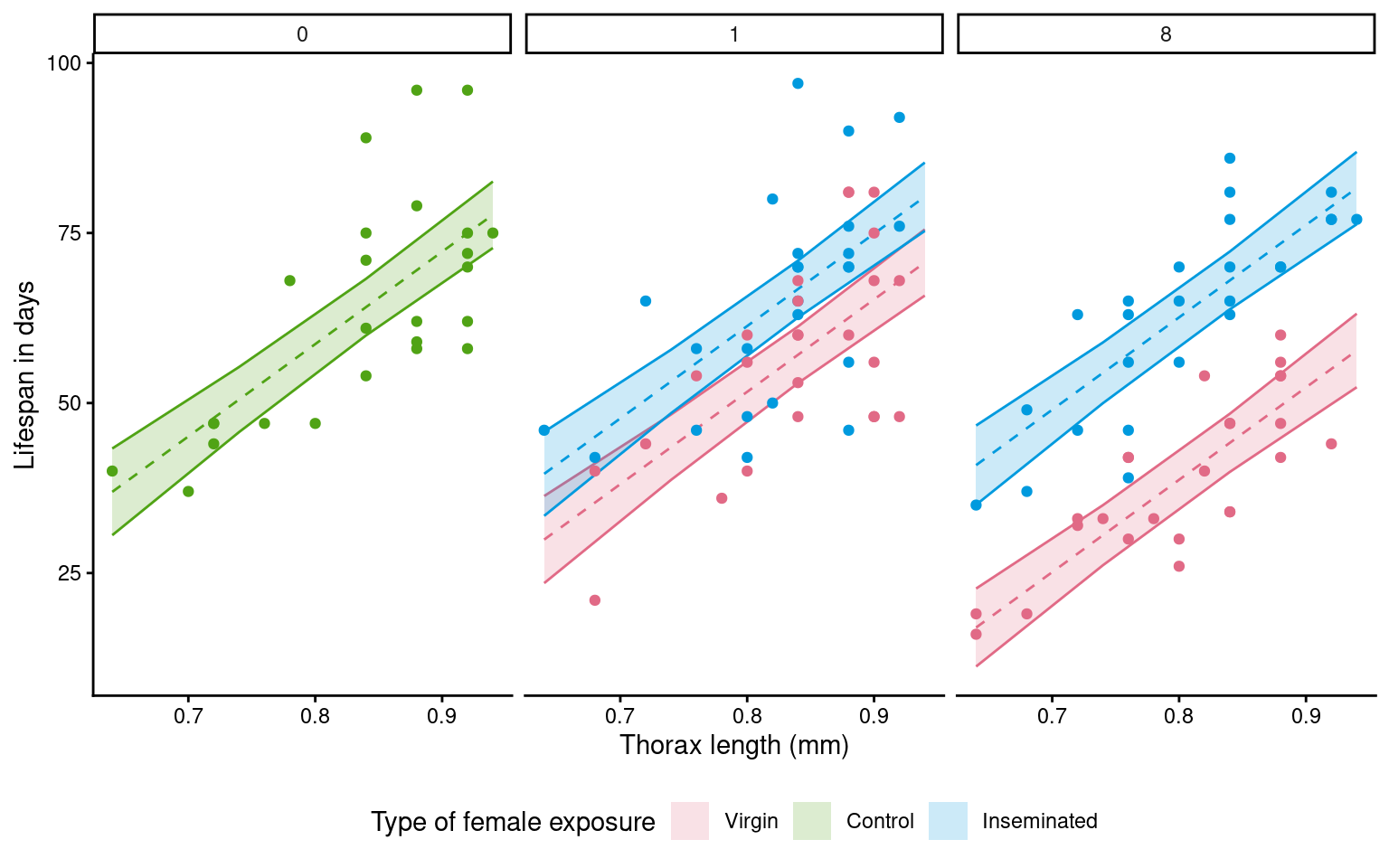
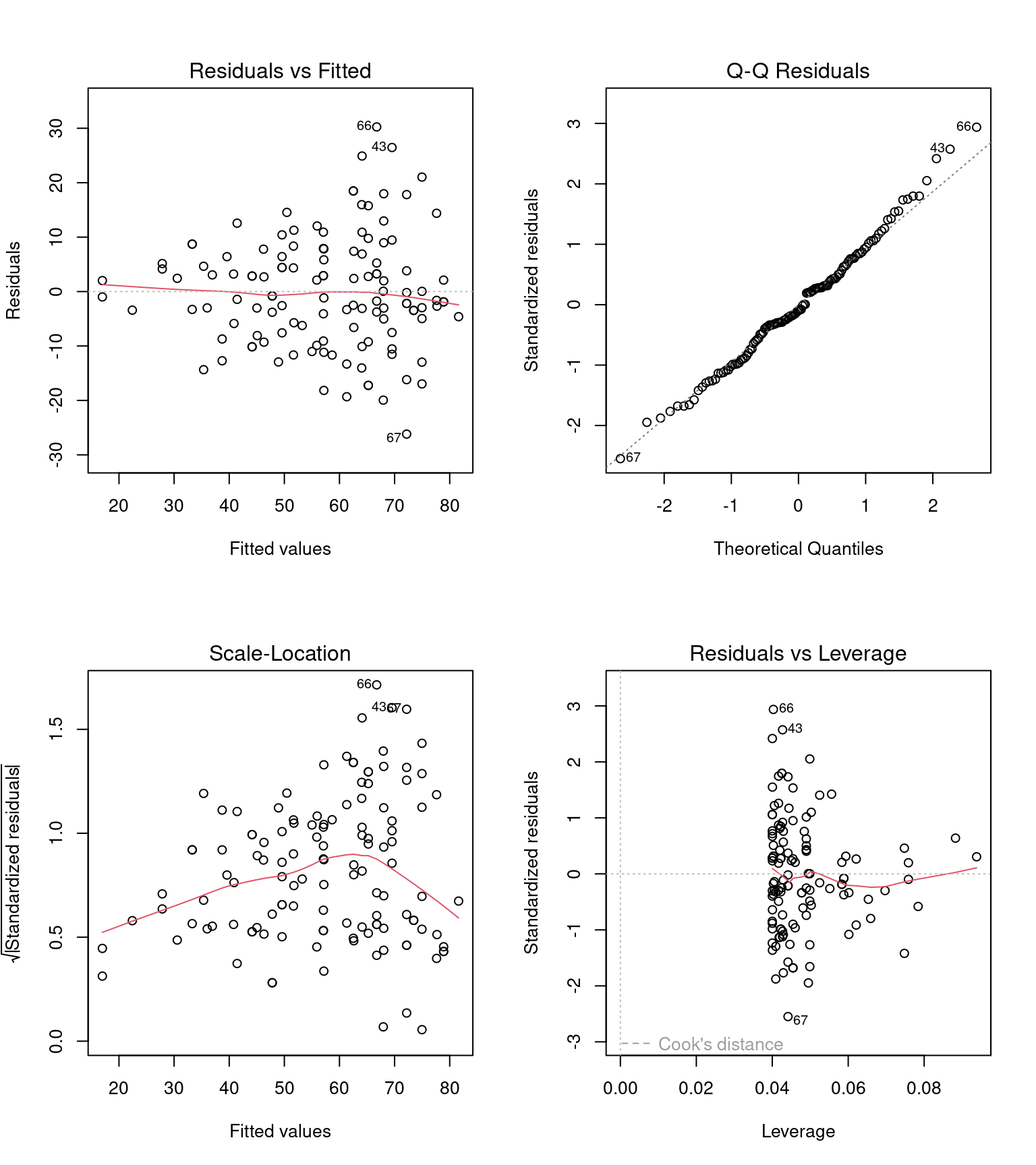
24.7 Model checking
Before we can interpret the terms in our model, we should check to see if this is even a good way of fitting and measuring our data. We should check the assumptions of our model are being met.
R has ways to do this with the plot() function, but the performance packages Lüdecke et al. (2025) from easystats also gives nice residual checks:
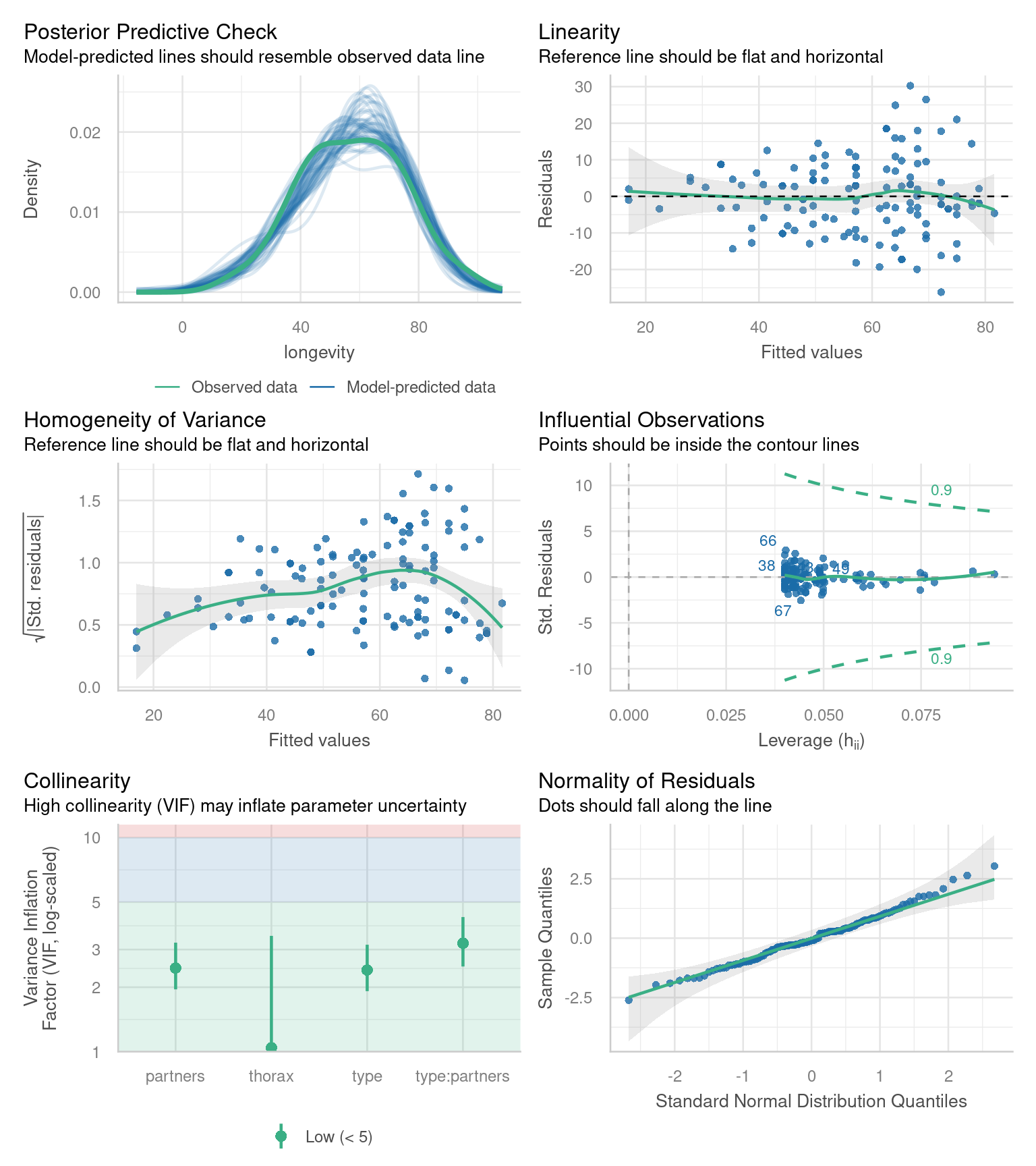
Posterior Predictive Check – Assesses whether the model’s predicted values align well with the observed data, indicating good model fit.
Linearity Check – Ensures that the relationship between predictor variables and the outcome is approximately linear, a key assumption of linear regression.
Homogeneity of Variance Check – Tests whether residuals (errors) have constant variance across all levels of predictors, known as homoscedasticity.
Influential Observation Check – Identifies individual data points that have a disproportionately large impact on the model’s estimates.
Collinearity Check – Detects whether predictor variables are highly correlated with each other, which can distort model estimates and reduce interpretability.
Normality Check – Examines whether the residuals of the model follow a normal distribution, an assumption necessary for reliable inference in linear regression.
24.7.1 Homogeneity of variance
Question - IS the assumption of homogeneity of variance met?
Mostly - the reference line is fairly flat (there is a slight curve).
It looks as though there might be some increasing heterogeneity with larger values, though very minor.
VERDICT, pretty much ok, should be fine for making inferences.
With a slight curvature this could indicate that you might get a better fit with a transformation, or perhaps that there is a missing variable that if included in the model would improve the residuals. In this instance I wouldn’t be overly concerned. See here for a great explainer on intepreting residuals1.
24.7.2 Normality of residuals
Yes - the QQplot looks pretty good, a very minor indication of a right skew, but nothing to worry about.
[Interpreting QQ plots][What is a Quantile-Quantile (QQ) plot?]
24.7.3 Collinearity
Question - IS their an issue with Collinearity?
What does it mean to have (multi)collinearity?
This is when one or more predictors are correlated - leading to increased uncertainty about their contributions to the outcome variable.
The result is wider standard error and confidence intervals.
While there are many discussions about what can be done with multicollinearity - I subscribed to the views outlined here.
It should be reported - but that’s it - it represents genuine uncertainty around the contributions of your predictors.
| Term | VIF | VIF_CI_low | VIF_CI_high | SE_factor | Tolerance | Tolerance_CI_low | Tolerance_CI_high |
|---|---|---|---|---|---|---|---|
| type | 2.407136 | 1.916931 | 3.159412 | 1.245590 | 0.4154314 | 0.3165146 | 0.5216672 |
| thorax | 1.042019 | 1.000713 | 3.475709 | 1.020793 | 0.9596755 | 0.2877111 | 0.9992873 |
| partners | 2.459411 | 1.954827 | 3.230645 | 1.252298 | 0.4066014 | 0.3095357 | 0.5115541 |
| type:partners | 3.208678 | 2.499097 | 4.254132 | 1.791278 | 0.3116548 | 0.2350656 | 0.4001445 |
https://www.qualtrics.com/support/stats-iq/analyses/regression-guides/interpreting-residual-plots-improve-regression/↩︎