6 Introduction to dplyr

6.1 Learning Objectives

By the end of this chapter, you will be able to:

Explain what the dplyr Wickham et al. (2023) package is and why it’s central to data wrangling.
Use the six core verbs of dplyr (select, filter, arrange, mutate, summarise, and group_by).
Chain multiple operations together using the pipe operator (|>).
Apply group_by() with summarise() to generate grouped summaries.

6.2 dplyr

The dplyr package (part of the tidyverse Wickham (2023)) provides simple, consistent functions for cleaning and transforming data. These are the building blocks for almost every data workflow in R. Once you understand these verbs, you can read and write tidy R code fluently.

Important

Try running the following functions directly in your consoleThe R console is the interactive interface within the R environment where users can type and execute R code. It is the place where you can directly enter commands, see their output, and interact with the R programming language in real-time.

6.3 Overview of Key Functions

verb	action
select()	choose columns by name
filter()	select rows based on conditions
arrange()	reorder the rows
summarise()	reduce raw data to user defined summaries
group_by()	group the rows by a specified column
mutate()	create a new variable

6.4 Select

If we wanted to create a dataset that only includes certain variables, we can use the dplyr::select() function from the dplyr package.

For example I might wish to create a simplified dataset that only contains species, sex, flipper_length_mm and body_mass_g.

Run the below code to select only those columns

select(
   # the data object
  .data = penguins_raw,
   # the variables you want to select
  `Species`, `Sex`, `Flipper Length (mm)`, `Body Mass (g)`)

Alternatively you could tell R the columns you don’t want e.g.

select(.data = penguins_raw,
       -`studyName`, -`Sample Number`)

Assign outputs

Note that select() does not change the original penguins tibble. It spits out the new tibble directly into your console.

If you don’t save this new tibble, it won’t be stored. If you want to keep it, then you must create a new object.

penguin_idcols <- select(.data = penguins_raw,
       -`studyName`, -`Sample Number`)

Your turn

Create a new tibble containing only species, sex, flipper length and body mass.

new_penguins <- select(.data = penguins_raw, 
       `Species`, `Sex`, `Flipper Length (mm)`, `Body Mass (g)`)

6.5 Filter

Having previously used dplyr::select() to select certain variables, we will now use dplyr::filter() to select only certain rows or observations. For example only Adelie penguins.

We can do this with the equivalence operator ==

filter(.data = penguins_raw, 
       `Species` == "Adelie Penguin (Pygoscelis adeliae)")

We can use several different operators to assess the way in which we should filter our data that work the same in tidyverse or base R.

Boolean expressions
Operator	Name
A < B	less than
A <= B	less than or equal to
A > B	greater than
A >= B	greater than or equal to
A == B	equivalence
A != B	not equal
A %in% B	in

If you wanted to select all the Penguin species except Adelies, you use ‘not equals’.

filter(.data = penguins_raw, 
       `Species` != "Adelie Penguin (Pygoscelis adeliae)")

This is the same as

filter(.data = penguins_raw, 
       `Species` %in% c("Chinstrap penguin (Pygoscelis antarctica)",
                      "Gentoo penguin (Pygoscelis papua)")
       )

You can include multiple expressions within filter() and it will pull out only those rows that evaluate to TRUE for all of your conditions.

Your turn

Filter the data so that it contains only Adelie penguins where flipper length was measured as greater than 190mm.

filter(.data = penguins_raw, 
       `Species` == "Adelie Penguin (Pygoscelis adeliae)", 
       `Flipper Length (mm)` > 190)

6.6 Arrange

The function arrange() sorts the rows in the table according to the columns supplied. For example

arrange(.data = penguins_raw, 
        `Sex`)

The data is now arranged in alphabetical order by sex. So all of the observations of female penguins are listed before males.

You can also reverse this with desc()

arrange(.data = penguins_raw, 
        desc(`Sex`))

6.7 Mutate

Sometimes we need to create a new variable that doesn’t exist in our dataset. For example we might want to figure out what the flipper length is when factoring in body mass.

To create new variables we use the function mutate().

Note that as before, if you want to save your new column you must save it as an object. Here we are mutating a new column and attaching it to the new_penguins data oject.

penguins_new_col <- mutate(.data = new_penguins,
                     body_mass_kg = `Body Mass (g)`/1000)

Question

What happens to your data if you forget to assign the new object?

If you do not assign the output to an R object using <- (either a new name or overwriting the old tibble) then the output will just print into the console and will not be saved

6.8 Pipes

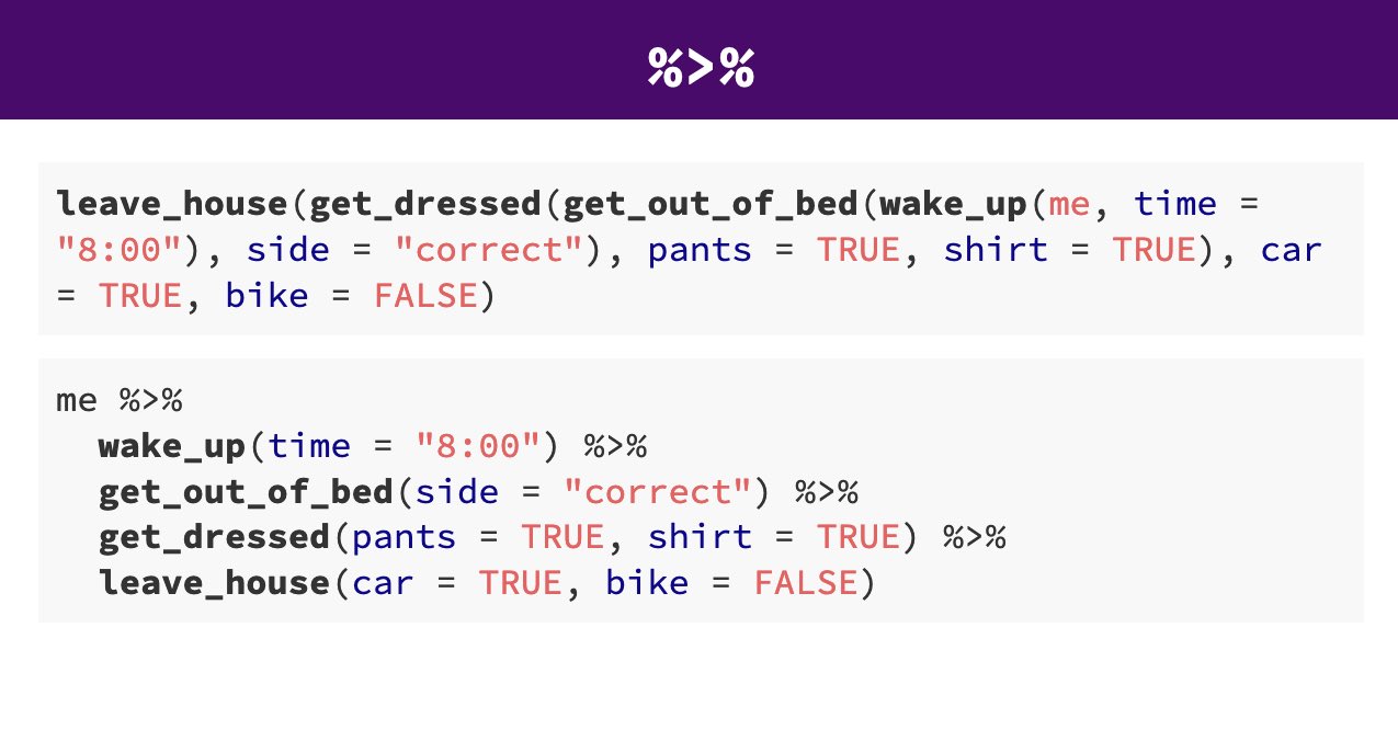
Pipes look like this: |> , a pipeAn operator that allows you to chain multiple functions together in a sequence. allows you to send the output from one function straight into another function. Specifically, they send the result of the function before |> to be the first argument of the function after |>. As usual, it’s easier to show, rather than tell so let’s look at an example.

# this example uses brackets to nest and order functions
arrange(.data = filter(
  .data = select(
  .data = penguins_raw, 
  species, `Sex`, `Flipper Length (mm)`), 
  `Sex` == "MALE"), 
  desc(`Flipper Length (mm)`))

# this example uses sequential R objects 
object_1 <- select(.data = penguins_raw, 
                   `Species`, `Sex`, `Flipper Length (mm)`)
object_2 <- filter(.data = object_1, 
                   `Sex` == "MALE")
arrange(object_2, 
        desc(`Flipper Length (mm)`))

# this example is human readable without intermediate objects
penguins_raw |>  
  select(`Species`, `Sex`, `Flipper Length (mm)`) |>  
  filter(`Sex` == "MALE") |>  
  arrange(`Flipper Length (mm)`)

The reason that this function is called a pipe is because it ‘pipes’ the data through to the next function. When you wrote the code previously, the first argument of each function was the dataset you wanted to work on. When you use pipes it will automatically take the data from the previous line of code so you don’t need to specify it again.

Your turn

Take any command you wrote earlier and rewrite it using pipes.

Native pipe |> and Magrittr %>%

From R version 4 onwards there is now a “native pipe” |>

This doesn’t require the tidyverse magrittr package and the “old pipe” %>% or any other packages to load and use.

You may be familiar with the magrittr pipe or see it in other tutorials, and website usages. The native pipe works equivalntly in most situations but if you want to read about some of the operational differences, this site does a good job of explaining .

Your turn

Check your RStudio settings to see if you are using the Native Pipe

Tools > Project Options > Code Editing > Use Native Pipe
The Shortcut key is (Ctrl/Cmd) + Shift + M

6.9 Group by

The group_by() function is used to tell R that you want to perform operations within groups of your data rather than across the whole dataset.

Think of it as adding a “temporary label” to each row that says which group it belongs to. Then, when you use functions like summarise(), R performs the summary for each group separately.

Let’s say you want to find the average flipper length for each penguin species.

Without grouping we get a single value:

penguins_raw |>  
  summarise(mean_flipper = mean(`Flipper Length (mm)`, na.rm = TRUE))

mean_flipper
200.9152

With grouping:

Gives one number per species

penguins_raw |> 
  group_by(`Species`) |> # select our variable that contains the groups
  summarise(mean_flipper = mean(`Flipper Length (mm)`, na.rm = TRUE),
            .groups = "drop" ) # remove groups after calculation

Species	mean_flipper
Adelie Penguin (Pygoscelis adeliae)	189.9536
Chinstrap penguin (Pygoscelis antarctica)	195.8235
Gentoo penguin (Pygoscelis papua)	217.1870

6.9.1 Grouping by multiple variables

penguins_raw |> 
  group_by(`Species`, `Sex`) |> 
  summarise(mean_flipper = mean(`Flipper Length (mm)`, na.rm = TRUE),
            .groups = "drop")

Species	Sex	mean_flipper
Adelie Penguin (Pygoscelis adeliae)	FEMALE	187.7945
Adelie Penguin (Pygoscelis adeliae)	MALE	192.4110
Adelie Penguin (Pygoscelis adeliae)	NA	185.6000
Chinstrap penguin (Pygoscelis antarctica)	FEMALE	191.7353
Chinstrap penguin (Pygoscelis antarctica)	MALE	199.9118
Gentoo penguin (Pygoscelis papua)	FEMALE	212.7069
Gentoo penguin (Pygoscelis papua)	MALE	221.5410
Gentoo penguin (Pygoscelis papua)	NA	215.7500

Note

You can think of group_by() as sorting your dataset into bins, one bin per group. Then, when you summarise() or mutate(), you’re performing that operation inside each bin.