20 Regression

20.1 Introduction to Regression

So far we have used linear models for analyses between two ‘categorical’ explanatory variables e.g. t-tests. But what about when we have a ‘continuous’ explanatory variable? For that we need to use a regression analysis, luckily this is just another ‘special case’ of the linear model, so we can use the same lm() function we have already been using, and we can interpret the outputs in the same way.

library(tidyverse)
library(here)
library(performance)

20.2 Linear regression

Much like the t-test we have generating from our linear model, the regression analysis is interpreting the strength of the ‘signal’ (the change in mean values according to the explanatory variable), vs the amount of ‘noise’ (variance around the mean).

We would normally visualise a regression analysis with a scatter plot, with the explanatory (predictor, independent) variable on the x-axis and the response (dependent) variable on the y-axis. Individual data points are plotted, and we attempt to draw a straight-line relationship throught the cloud of data points. This line is the ‘mean’, and the variability around the mean is captured by calculated standard errors and confidence intervals from the variance.

The equation for the linear regression model is:

\[ y = a + bx \] You may also note this is basically identical to the equation for a straight fit line \(y = mx +c\).

Here:

y is the predicted value of the response variable
a is the regression intercept (the value of y when x = 0)
b is the slope of the regression line
x is the value of the explanatory variable

This formula explains the mean, you would need to include the unexplained residual error as a term to include our measure of uncertainty

\[ y = a + bx + e \]

The regression uses two values to fit a straight line. First we need a starting point, known as the regression intercept. For categorical predictors this is the mean value of y for one of our categories, for a regression this is the mean value of y when x = 0. We then need a gradient (how the value of y changes when the value of x changes). This allows us to draw a regression line.

A linear model analysis estimates the values of the intercept and gradient in order to predict values of y for given values of x.

20.3 Data

Here we are going to use example data from the Australian forestry industry, recording the density and hardness of 36 samples of wood from different tree species. Wood density is a fundamental property that is relatively easy to measure, timber hardness, is quantified as the ‘the amount of force required to embed a 0.444” steel ball into the wood to half of its diameter’.

With regression, we can test the biological hypothesis that wood density can be used to predict timber hardness, and use this regression to predict timber hardness for new samples of known density.

Timber hardness is quantified using the ‘Janka scale’, and the data we are going to use today comes originally from an R package SemiPar

janka <- read_csv(here("data", "clean", "janka.csv")

20.4 Exploratory Analysis & Correlation

Your turn

Make a plot. Is there any visual evidence for a linear association between wood density and timber hardness?

janka |> 
  ggplot(aes(x=dens, y=hardness))+
  geom_point()

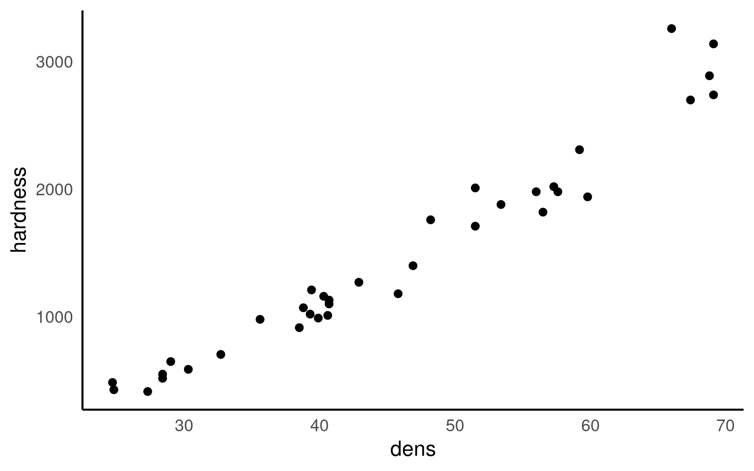
Wood density and timber hardness appear to be positively related, and the relationship appears to be fairly linear. We can look at a simple strength of this association between dens and hardness using correlation

Can you work out the code needed to generate a correlation coefficient?

Hint see Section 16.8

janka |> 
  summarise(cor(dens,
                hardness),
            n = n())

cor(dens, hardness)	n
0.9743345	36

Correlation coefficients range from -1 to 1 for perfectly negative to perfectly positive linear relationships. The relationship here appears to be strongly positive. Correlation looks at the association between two variables, but we want to go further - we are arguing that wood density causes higher values of timber hardness. In order to test that hypothesis we need to go further than correlation and use regression.

20.5 Regression in R

We can fit the regression model in exactly the same way as we fit the linear model for Darwin’s maize data. The only difference is that here our predictor variable is continuous rather than categorical.

janka_ls1 <- lm(hardness ~ dens, data = janka)

This linear model will estimate a ‘line of best fit’ using the method of ‘least squares’ to minimise the error sums of squares (the average distance between the data points and the regression line).

Be careful when ordering variables here:

the left of the ‘tilde’ is the response variable,
on the right is the predictor.

Get them the wrong way round and it will reverse your hypothesis.

We can add a regression line to our ggplots very easily with the function geom_smooth().

When we specify the argument method = lm we restrict line fitting to an OLS regression

# specify linear model method for line fitting

janka |> 
  ggplot(aes(x=dens, y=hardness))+
  geom_point()+
  geom_smooth(method="lm")

Note

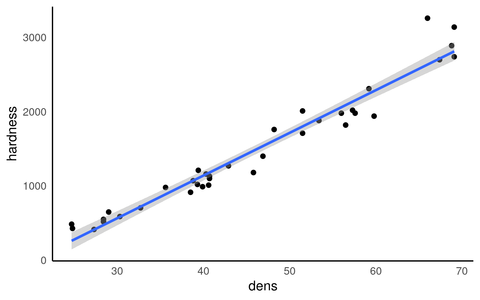
geom_smooth() is a simple way to plot regressions, but it is limited to single predictor models, and should not be used for more complex analyses

20.5.0.1 Summary

summary(janka_ls1)


Call:
lm(formula = hardness ~ dens, data = janka)

Residuals:
    Min      1Q  Median      3Q     Max 
-338.40  -96.98  -15.71   92.71  625.06 

Coefficients:
             Estimate Std. Error t value Pr(>|t|)    
(Intercept) -1160.500    108.580  -10.69 2.07e-12 ***
dens           57.507      2.279   25.24  < 2e-16 ***
---
Signif. codes:  0 '***' 0.001 '**' 0.01 '*' 0.05 '.' 0.1 ' ' 1

Residual standard error: 183.1 on 34 degrees of freedom
Multiple R-squared:  0.9493,    Adjusted R-squared:  0.9478 
F-statistic:   637 on 1 and 34 DF,  p-value: < 2.2e-16

janka_ls1 |> 
  broom::tidy()

term	estimate	std.error	statistic	p.value
(Intercept)	-1160.49970	108.579605	-10.68801	0
dens	57.50667	2.278534	25.23845	0

This output should look very familiar to you, because it’s the same output produced for the analysis of the maize data. Including a column for the coefficient estimates, standard error, t-statistic and P-value. The first row is the intercept, and the second row is the difference in the mean from the intercept caused by our explanatory variable.

In a test of difference, the intercept represented the mean of one group and the coefficient tells you how much higher or lower the average of one group is compared to another group.
In regression analysis, the intercept is the value when the predictor variable is zero and the coefficient shows how much the response variable changes when the predictor variable increases by one unit, while keeping other predictors constant. This might mean the effect looks small - but it is cumulative.

20.6 Mean-centering

In many ways the intercept makes more intuitive sense in a regression model than a difference model.

Here the intercept describes the value of y (timber hardness) when x (wood density) = 0. The standard error is the standard error of this calculated mean value. The only wrinkle here is that that value of y is an impossible value - timber hardness obviously cannot be a negative value (anti-hardness???). This does not affect the fit of our line, it just means a regression line (being an infinite straight line) can move into impossible value ranges.
One way in which the intercept can be made more valuable is to use a technique known as mean-centering. By subtracting the average (mean) value of x from every data point, the intercept (when x is 0) can effectively be right-shifted into the centre of the data. This is known as mean-centered regression

Your turn

Can you use your data wrangling skills to mean centre the density predictor and produce a more realistic model intercept?

Compare the two models, what is the same and what has changed?

janka_centered <-  janka |> 
  mutate(centered_dens = dens - mean(dens)) 
# mutate creates a new column where each value of dens is subtracted from the overall mean

centered_model <- lm(hardness ~ centered_dens, data = janka_centered) 
# model uses the new variable

summary(centered_model)


Call:
lm(formula = hardness ~ centered_dens, data = janka_centered)

Residuals:
    Min      1Q  Median      3Q     Max 
-338.40  -96.98  -15.71   92.71  625.06 

Coefficients:
              Estimate Std. Error t value Pr(>|t|)    
(Intercept)   1469.472     30.510   48.16   <2e-16 ***
centered_dens   57.507      2.279   25.24   <2e-16 ***
---
Signif. codes:  0 '***' 0.001 '**' 0.01 '*' 0.05 '.' 0.1 ' ' 1

Residual standard error: 183.1 on 34 degrees of freedom
Multiple R-squared:  0.9493,    Adjusted R-squared:  0.9478 
F-statistic:   637 on 1 and 34 DF,  p-value: < 2.2e-16

summary(janka_ls1)


Call:
lm(formula = hardness ~ dens, data = janka)

Residuals:
    Min      1Q  Median      3Q     Max 
-338.40  -96.98  -15.71   92.71  625.06 

Coefficients:
             Estimate Std. Error t value Pr(>|t|)    
(Intercept) -1160.500    108.580  -10.69 2.07e-12 ***
dens           57.507      2.279   25.24  < 2e-16 ***
---
Signif. codes:  0 '***' 0.001 '**' 0.01 '*' 0.05 '.' 0.1 ' ' 1

Residual standard error: 183.1 on 34 degrees of freedom
Multiple R-squared:  0.9493,    Adjusted R-squared:  0.9478 
F-statistic:   637 on 1 and 34 DF,  p-value: < 2.2e-16

We should note that our slope of regression and the statistics associated with it are unchanged - that makes sense our relationship is unaltered. Only the starting point for drawing our straight line (the intercept) has moved.

20.6.0.1 Confidence intervals

Just like with the maize data, we can produce upper and lower bounds of confidence intervals:

confint(janka_ls1)

                  2.5 %     97.5 %
(Intercept) -1381.16001 -939.83940
dens           52.87614   62.13721

broom::tidy(janka_ls1, conf.int=T, conf.level=0.95)

term	estimate	std.error	statistic	p.value	conf.low	conf.high
(Intercept)	-1160.49970	108.579605	-10.68801	0	-1381.16001	-939.83940
dens	57.50667	2.278534	25.23845	0	52.87614	62.13721

What would you say is the minimum effect size (at 95% confidence) of density on the janka scale?

Here we can say that at \(\alpha\) = 0.05 we think the mean change is at least a 52.9 unit increase on the janka scale for every unit increase in density.

Because our 95% confidence intervals do not span 0, we can also say that there is a significant relationship at \(\alpha\) < 0.05.

20.6.1 Effect size

With a regression model, we can also produce a standardised effect size. The estimate and 95% confidence intervals are the amount of change being observed, but just like with the maize data we can produce a standardised measure of how strong the relationship is. This value is represented by \(R^2\) : the proportion of the variation in the data explained by the linear regression analysis.

The value of \(R^2\) can be found in the model summaries as follows

summary(janka_ls1)


Call:
lm(formula = hardness ~ dens, data = janka)

Residuals:
    Min      1Q  Median      3Q     Max 
-338.40  -96.98  -15.71   92.71  625.06 

Coefficients:
             Estimate Std. Error t value Pr(>|t|)    
(Intercept) -1160.500    108.580  -10.69 2.07e-12 ***
dens           57.507      2.279   25.24  < 2e-16 ***
---
Signif. codes:  0 '***' 0.001 '**' 0.01 '*' 0.05 '.' 0.1 ' ' 1

Residual standard error: 183.1 on 34 degrees of freedom
Multiple R-squared:  0.9493,    Adjusted R-squared:  0.9478 
F-statistic:   637 on 1 and 34 DF,  p-value: < 2.2e-16

janka_ls1 |> 
  broom::glance()

r.squared	adj.r.squared	sigma	statistic	p.value	df	logLik	AIC	BIC	deviance	df.residual	nobs
0.9493278	0.9478374	183.0595	636.9794	0	1	-237.6061	481.2123	485.9628	1139366	34	36

20.7 Prediction

Using the coefficients of the intercept and the slope we can make predictions on new data.

The estimates of the intercept and the slope are:

coef(janka_ls1)

(Intercept)        dens 
-1160.49970    57.50667

Now imagine we have a new wood samples with a density of 70, how can we use the equation for a linear regression to predict what the timber hardness for this wood sample should be?

\[ y = a + bx \]

# a + bx

-1160.49970 + 57.50667 * 70

[1] 2864.967

Rather than work out the values manually, we can also use the coefficients of the model directly

coef(janka_ls1)[1] + coef(janka_ls1)[2] * 70

(Intercept) 
   2864.968

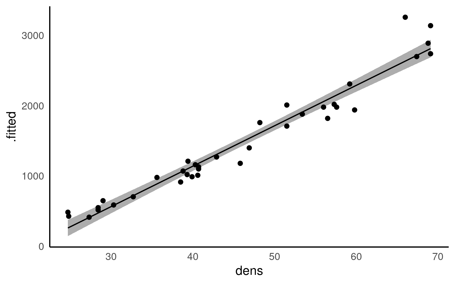
Most of the time we are unlikely to want to work out predicted values by hand, instead we can use functions like predict() and broom::augment()

predict(janka_ls1, newdata=list(dens=c(22,35,70)))

        1         2         3 
 104.6471  852.2339 2864.9675

broom::augment(janka_ls1, 
               newdata=tibble(dens=c(22,35,70)))

dens	.fitted
22	104.6471
35	852.2339
70	2864.9675

20.7.1 Adding confidence intervals

20.7.1.1 Standard error

broom::augment(janka_ls1, 
               newdata = tibble(dens=c(22,35,70)), 
               se=TRUE)

dens	.fitted	.se.fit
22	104.6471	62.09026
35	852.2339	39.10197
70	2864.9675	63.15147

20.7.1.2 95% Confidence Intervals

broom::augment(janka_ls1, 
               newdata=tibble(dens=c(22,35,70)), 
               interval="confidence")

dens	.fitted	.lower	.upper
22	104.6471	-21.53544	230.8297
35	852.2339	772.76915	931.6987
70	2864.9675	2736.62830	2993.3068

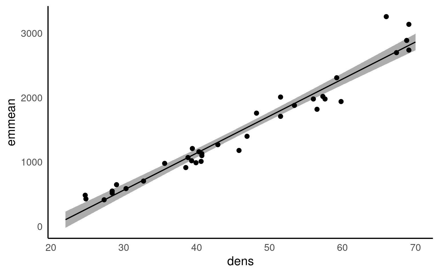
I really like the emmeans::emmeans() function - it is very good for producing quick predictions for categorical data - it can also do this for continuous variables. By default it will produce a single mean-centered prediction. But a list can be provided - it will produce confidence intervals as standard.

emmeans::emmeans(janka_ls1, 
                 specs = "dens", 
                 at = list(dens = c(22, 
                                    35, 
                                    70)))

 dens emmean   SE df lower.CL upper.CL
   22    105 62.1 34    -21.5      231
   35    852 39.1 34    772.8      932
   70   2865 63.2 34   2736.6     2993

Confidence level used: 0.95

emmeans::emmeans(janka_ls1, 
                 specs = "dens", 
                 at = list(dens = seq (from = 22,
                                       to = 70,
                                      by = 1)))

 dens emmean   SE df lower.CL upper.CL
   22    105 62.1 34    -21.5      231
   23    162 60.1 34     40.0      284
   24    220 58.2 34    101.5      338
   25    277 56.2 34    162.9      391
   26    335 54.3 34    224.2      445
   27    392 52.5 34    285.6      499
   28    450 50.6 34    346.8      553
   29    507 48.8 34    408.0      606
   30    565 47.1 34    469.0      660
   31    622 45.4 34    530.0      714
   32    680 43.7 34    590.9      769
   33    737 42.1 34    651.7      823
   34    795 40.6 34    712.3      877
   35    852 39.1 34    772.8      932
   36    910 37.7 34    833.1      986
   37    967 36.4 34    893.2     1041
   38   1025 35.2 34    953.2     1096
   39   1082 34.2 34   1012.9     1152
   40   1140 33.2 34   1072.3     1207
   41   1197 32.4 34   1131.5     1263
   42   1255 31.7 34   1190.4     1319
   43   1312 31.1 34   1249.0     1376
   44   1370 30.8 34   1307.3     1432
   45   1427 30.6 34   1365.2     1489
   46   1485 30.5 34   1422.8     1547
   47   1542 30.6 34   1480.0     1605
   48   1600 30.9 34   1536.9     1663
   49   1657 31.4 34   1593.5     1721
   50   1715 32.0 34   1649.8     1780
   51   1772 32.8 34   1705.7     1839
   52   1830 33.7 34   1761.4     1898
   53   1887 34.7 34   1816.8     1958
   54   1945 35.9 34   1872.0     2018
   55   2002 37.1 34   1927.0     2078
   56   2060 38.4 34   1981.7     2138
   57   2117 39.9 34   2036.3     2198
   58   2175 41.4 34   2090.8     2259
   59   2232 42.9 34   2145.1     2320
   60   2290 44.6 34   2199.3     2381
   61   2347 46.3 34   2253.4     2441
   62   2405 48.0 34   2307.4     2502
   63   2462 49.8 34   2361.2     2564
   64   2520 51.6 34   2415.1     2625
   65   2577 53.5 34   2468.8     2686
   66   2635 55.3 34   2522.5     2747
   67   2692 57.3 34   2576.1     2809
   68   2750 59.2 34   2629.6     2870
   69   2807 61.2 34   2683.2     2932
   70   2865 63.2 34   2736.6     2993

Confidence level used: 0.95

20.8 Results

Your turn

Can you write a summary of the Results?
Make a prediction plot from the fitted model

Hint - use augment or emmeans to make your predictions and 95%CI - try to add raw data to the plot as well.

Remember if using emmeans it must be converted to a tibble for plotting

We analysed the relationship between wood density and timber hardness on the janka scale with a linear regression model and found that wood density is an excellent predictor of timber harndess (R^2 = 0.95). With an average wood density of 45.7, this produced a timber hardness of 1469 [1407, 1531] (mean [95% CI]) on the janka scale, and for every unit of density, timber hardness increases by 57.5 [52.9, 62.1] (t(34) = 25.24, p <0.001).

broom::augment(janka_ls1,
               interval="confidence") |> 
  ggplot(aes(x = dens,
             y = .fitted))+
  geom_ribbon(aes(ymin = .lower,
                  ymax = .upper),
              alpha = .4)+
  geom_line()+
  geom_point(aes(x = dens,
                 y = hardness))

emmeans::emmeans(janka_ls1, 
                 specs = "dens", 
                 at = list(dens = seq(22, 70, by = 1))) |> 
  as_tibble() |> 
    ggplot(aes(x = dens,
             y = emmean))+
  geom_ribbon(aes(ymin = lower.CL,
                  ymax = upper.CL),
              alpha = .4)+
  geom_line()+
  geom_point(data = janka,
    aes(x = dens,
        y = hardness))

20.9 Summary

Linear model analyses can extend beyond testing differences of means in categorical groupings to test relationships with continuous variables. This is known as linear regression, where the relationship between the explanatory variable and response variable are modelled with the equation for a straight line. The intercept is the value of y when x = 0, often this isn’t that useful, and we can use ‘mean-centered’ values if we wish to make the intercept more intuitive. As with all linear models, regression assumes that the unexplained variability around the regression line, is normally distributed and has constant variance.

Once the regression has been fitted it is possible to predict values of y from values of x, the uncertainty around these predictions can be captured with confidence intervals.

20.10 Assumption checking

After conducting a linear model analysis, we often find ourselves with results and inferences. However, before we can fully trust our analysis, it’s essential to check whether the underlying assumptions of the model are adequately met.

check_model(janka_ls1,
            detrend = FALSE,
            check = c("linearity",
                       "homogeneity",
                       "outliers",
                       "qq"))

Based on these residual checks - what do you think the main issues with the model are?

We begin by fitting a linear regression model to examine the relationship between wood density and timber hardness. The model explains a large proportion of the variance in the outcome (high R squared), indicating a strong predictive association. But there are some minor issues with the model to consider:

Non-linearity: there is a pattern of curvature in the residuals indicating the relationship is not strictly linear
Heteroscedasticty: The residual plots indicate increasing spread of the residuals as fitted values increase - this will affect standard errors, 95%CI and p-values
One observation has high leverage and influences the fitted line

Taken together the diagnostics indicate the model violates some key assumptions underlying linear regression. We might consider nonlinear terms or data transformations - which we can cover later.