Appendix E — Quarto

Quarto is a new and improved version of RMarkdown that makes working with different formats and programming languages easier. If you have ever used RMarkdown, the transition is easy.

One of the main benefits of Quarto is that it uses a consistent set of rules across all types of output. In R Markdown, the way you format documents can change depending on what you are creating. For example, when making slides in R Markdown, the “xaringan” package uses three dashes to create new slides, but in other formats, three dashes create a horizontal line instead. Similarly, the “distill” package has its own unique layout options that don’t work with “xaringan.” Quarto simplifies this by providing one standard way to format all types of documents.

Quarto also supports more programming languages than R Markdown and works with different code editors. While R Markdown is mainly designed to be used in the RStudio program, Quarto can be used not only in RStudio but also in other popular code editors, like Visual Studio (VS) Code and JupyterLab. This makes it easier for people to use Quarto with different languages and tools.

This chapter will show you the benefits of using Quarto if you are an R user. It will guide you on how to set up Quarto, explain the key differences between Quarto and R Markdown, and teach you how to use Quarto to create reports, presentations, and websites.

E.1 Background

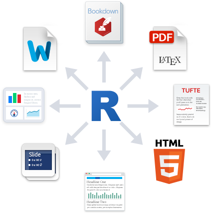
Quarto is a widely-used tool for creating automated, reproducible, and share-worthy outputs, such as reports. It can generate static or interactive outputs, in Word, pdf, html, Powerpoint slides, and many other formats.

A Quarto file combines R code (or other programming code) and text such that the script actually becomes your output document. You can create an entire formatted document, including narrative text (can be dynamic to change based on your data), tables, figures, bullets/numbers, bibliographies, etc.

Documents produced with Quarto, allow analyses to be included easily - and make the link between raw data, analysis & and a published report completely reproducible.

With Quarto we can make reproducible html, word, pdf, powerpoints or websites and dashboards¹

How it works

Starting from version 2022.07.1, RStudio comes with Quarto already installed.

To check which version of RStudio you have, go to the top menu and click on RStudio > About RStudio. If your version is older than 2022.07.1, you should update it by reinstalling RStudio. Instructions for updating RStudio can be found in Chapter 1. After updating, Quarto should be automatically installed.

Once Quarto is installed, you can create a new document by clicking File > New File > Quarto Document. This will bring up a menu similar to the one used to create an R Markdown document

Choose a title, author, as well as your default output format (HTML, PDF, or Word). These values can be changed later. Click OK, and RStudio will create a Quarto document with some placeholder content.

This document contains several sections, each of which we will discuss below. First, though, let’s skip to the finish line by doing what’s called rendering our document. The Render button at the top of RStudio converts the Quarto document into whatever format we selected.

To make your document publish - hit the render button at the top of the doc

Quarto parts

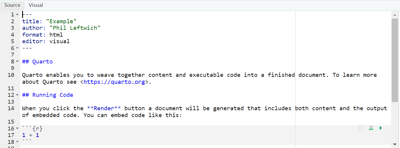
Tip

Rstudio lets you view your Quarto document in visual (partially rendered) or source (all plain text) mode. The code and explanations below work best if you are viewing in source

As you can see, there are three basic components to any Quarto file:

YAML
Markdown text
R code chunks.

YAML Metadata

The YAML section is the very beginning of an R Markdown document. The name YAML comes from the recursive acronym YAML ain’t markup language, whose meaning isn’t important for our purposes. Three dashes indicate its beginning and end, and the text inside of it contains metadata about the R Markdown document. Here is my YAML:


---
title: "My Report"
output: html_document
---

As you can see, it provides the title, author, and output format. All elements of the YAML are given in key: value syntax, where each key is a label for a piece of metadata (for example, the title) followed by a value in quotes.

In the example above, because we clicked that our default output would be an html file, we can see that the YAML says output: html. However we can also change this to say pptx or docx or even pdf_document. (https://quarto.org/docs/output-formats/all-formats.html)

E.1.1 TASK: Can you edit the YAML in the Rmarkdown file in the markdown folder to have your name as author? Try changing the output to a different file type.

Code chunks

Quarto documents have a different structure from the R script files you might be familiar with (those with the .R extension). R script files treat all content as code unless you comment out a line by putting a pound sign (#) in front of it. In the following code, the first line is a comment while the second line is code.


```{r}
# Import our data
data <- read_csv("data.csv")
```

In Quarto, the situation is reversed. Everything after the YAML is treated as text unless we specify otherwise by creating what are known as code chunks. Each chunk is opened with a line that starts with three back-ticks, and curly brackets that contain parameters for the chunk { }. The chunk ends with three more back-ticks.


```{r}
library(tidyverse)
```

Quarto treats anything in the code chunk as R code when we knit. For example, this code chunk will produce a histogram in the final document.


```{r}

hist(cars$speed)
```

Some notes about the contents of the curly brackets { }:

They start with ‘r’ to indicate that the language name within this chunk is R. It is possible to include other programming language chunks here such as SQL, Python or Bash.

After the r you can optionally write a chunk “name” – these are not necessary but can help you organise your work. Note that if you name your chunks, you should ALWAYS use unique names or else R will complain when you try to render.

After the language name and optional chunk name put a comma, then you can include other options too, written as tag=value, such as:

eval: false to not run the R code
echo: false to not print the chunk’s R source code in the output document
warning: false to not print warnings produced by the R code
message: false to not print any messages produced by the R code
include: true/false whether to include chunk outputs (e.g. plots) in the document
out-width and out-height = size of output in final document e.g. out-width = “75%”
fig-width and fig-height: relative size of figure
fig-align = “center” adjust how a figure is aligned across the page
fig-show=‘hold’ if your chunk prints multiple figures and you want them printed next to each other (pair with out-width = c(“33%”, “67%”).

Question. If we wanted to see the R code, but not its output we need to select what combo of code chunk options?

Default options for showing code, charts, and other elements in the rendered versions of the document. In Quarto, these options are set in the execute field of the YAML. For example, the following would provide the outputs of code, but hide the code itself, as well as all warnings and messages, from the rendered document:

---
title: "My Report"
format: html
execute:
  echo: false
  warning: false
  message: false
---

In cases where you’re using Quarto to generate a report for a non-R user, you likely want to follow this setup of hiding the code, messages, and warnings but show the output (which would include any visualizations you generate).

However, you can also override these global code chunk options on individual chunks. If I wanted my document to show both the plot itself and the code used to make it, I could set echo = TRUE for that code chunk only:


```{r}
#| echo = TRUE
hist(cars$speed)
```

The option is set within the code chunk itself. The characters #| (known as a hash pipe) at the start of a line indicate that you are setting options.

Text

This is the narrative of your document, including the titles and headings. It is written in the “markdown” language, which is used across many different software.

Below are the core ways to write this text. See more extensive documentation available on R Markdown “cheatsheets” at the RStudio website².

Text emphasis

Surround your normal text with these characters to change how it appears in the output.

Underscores (_text_) or single asterisk (*text*) to italicise

Double asterisks (**text**) for bold text

Back-ticks (` text `) to display text as code

The actual appearance of the font can be set by using specific templates (specified in the YAML metadata).

Titles and headings

A hash symbol in a text portion of a R Markdown script creates a heading. This is different than in a chunk of R code in the script, in which a hash symbol is a mechanism to comment/annotate/de-activate, as in a normal R script.

Different heading levels are established with different numbers of hash symbols at the start of a new line. One hash symbol is a title or primary heading. Two hash symbols are a second-level heading. Third- and fourth-level headings can be made with successively more hash symbols.


# First-level heading / Title

## Second level heading  

### Third-level heading

Bullets and numbering

Use asterisks (*) to created a bullets list. Finish the previous sentence, enter two spaces, Enter/Return twice, and then start your bullets. Include a space between the asterisk and your bullet text. After each bullet enter two spaces and then Enter/Return. Sub-bullets work the same way but are indented. Numbers work the same way but instead of an asterisk, write 1), 2), etc. Below is how your R Markdown script text might look.

Here are my bullets (there are two spaces after this colon):

* Bullet 1 (followed by two spaces and Enter/Return)  
* Bullet 2 (followed by two spaces and Enter/Return)  
  * Sub-bullet 1 (followed by two spaces and Enter/Return)  
  * Sub-bullet 2 (followed by two spaces and Enter/Return)

In-text code

You can also include minimal R code within back-ticks. Within the back-ticks, begin the code with “r” and a space, so RStudio knows to evaluate the code as R code. See the example below.

This book was printed on `r Sys.Date()`

When typed in-line within a section of what would otherwise be Markdown text, it knows to produce an r output instead:

This book was printed on 2024-11-25

Running code

You can run the code in an R Markdown document in two ways. The first way is by rendering the entire document. The second way is to run code chunks manually (also known as interactively) by hitting the little green play button at the top-right of a code chunk. The down arrow next to the green play button will run all code until that point.

The one downside to running code interactively is that you can sometimes make mistakes that cause your Quarto document to fail to knit. That is because, in order to render, a Quarto document must contain all the code it uses. If you are working interactively and, say, load data from a separate file, you will be unable to knit your document. When working in R Markdown, always keep all code within a single document.

The code must also always appear in the right order.

E.2 Self contained Reports

For a relatively simple report, you may elect to organize your R Markdown script such that it is “self-contained” and does not involve any external scripts.

Set up your Rmd file to ‘read’ the penguins data file.

Everything you need to run the R markdown is imported or created within the Rmd file, including all the code chunks and package loading. This “self-contained” approach is appropriate when you do not need to do much data processing (e.g. it brings in a clean or semi-clean data file) and the rendering of the R Markdown will not take too long.

In this scenario, one logical organization of the R Markdown script might be:

Set global knitr options
Load packages
Import data
Process data
Produce outputs (tables, plots, etc.)
Save outputs, if applicable (.csv, .png, etc.)

E.2.1 TASK: Generate a self-contained report from data

Delete this content and replace it with your own. As an example, let’s create a report about penguins. Add the following content to a Quarto doc:

---
title: "Penguins Report"
author: "Phil"
output: html
execute:
  echo: false
  warning: false
  message: false
---

```{r}

library(tidyverse)

```

```{r}

penguins_raw <- read_csv(here::here("files", "penguins_raw.csv"))

```

# Introduction

We are writing a report about the **Palmer Penguins**. These penguins are *really* amazing. There are three species:

- Adelie
- Gentoo
- Chinstrap

## Bill Length

We can make a histogram to see the distribution of bill lengths.

```{r}
penguins_raw |> 
  ggplot(aes(x = `Culmen Length (mm)`)) +
  geom_histogram() +
  theme_minimal()
```

```{r}
average_bill_length <- penguins_raw |> 
  summarize(avg_bill_length = mean(`Culmen Length (mm)`,
                                   na.rm = TRUE)) |> 
  pull(avg_bill_length)
```

The chart shows the distribution of bill lengths. The average bill length is `r average_bill_length`.

ggplot

Size options for figures

fig.width and fig.height enable to set width and height of R produced figures. The default value is set to 7 (inches). When I play with these options, I prefer using only one of them (fig.width).
fig.asp sets the height-to-width ratio of the figure. It’s easier in my mind to play with this ratio than to give a width and a height separately. The default value of fig.asp is NULL but I often set it to (0.8), which often corresponds to the expected result.

Size options of figures produced by R have consequences on relative sizes of elements in this figures. For a ggplot2 figure, these elements will remain to the size defined in the used theme, whatever the chosen size of the figure. Therefore a huge size can lead to a very small text and vice versa.

The base font size is 11 pts by default. You can change it with the base_size argument in the theme you’re using.

penguin_colours <- c("darkolivegreen4", "darkorchid3", "goldenrod1")

plot <- penguins_raw |> 
  ggplot(aes(x=`Flipper Length (mm)`, 
             y = `Body Mass (g)`))+
  geom_point(aes(colour=`Species`))+
  scale_color_manual(values=penguin_colours)+
  theme_minimal(base_size = 11)

```{r fig.asp = 0.8, fig.width = 3}
plot
# figure elements are too big
```

```{r fig.asp = 0.8, fig.width = 10}
plot
# figure elements are too small
```

To find the result you like, you’ll need to combine sizes set in your theme and set in the chunk options. With my customised theme, the default size (7) looks good to me.

```{r fig.asp = 0.8, fig.width = 7}
plot
```

When texts axis are longer or when figures is overloaded, you can choose bigger size (8 or 9) to relatively reduce the figure elements. it’s worth noting that for the text sizes, you can also modify the base size in your theme to obtain similar figures.

```{r fig.asp = 0.8, fig.width = 7}
plot + theme(base_size = 14)
# figure width stays the same, but modify the text size in ggplot
```

Size of final figure in document

With the previous examples, you could see the relative size of the elements within the figures was changed - but the area occupied by the figures remained the same. In order to change this I need out.width or out.height

Figures made with R in a R Markdown document are exported (by default in png format) and then inserted into the final rendered document. Options out.width and out.height enable us to choose the size of the figure in the final document.

It is rare I need to re-scale height-to-width ratio after the figures were produced with R and this ratio is kept if you modify only one option therefore I only use out.width. i like to use percentage to define the size of output figures. For example hre with a size set to 50%

```{r fig.asp = 0.8, fig.width = 7, out.width = "50%"}
plot 
# The final rendered size of the image changes according to out.width
```

Static images

You can include images in your R Markdown:

```{r setup, include=FALSE}
knitr::include_graphics("path/to/image.png")
```

Tables

Markdown tables

| Syntax      | Description |
| ----------- | ----------- |
| Header      | Title       |
| Paragraph   | Text        |

Which will render as this

Syntax	Description
Header	Title
Paragraph	Text

gt()

The gt Iannone et al. (2025) package is all about making it simple to produce nice-looking display tables. It has a lot of customisation options.

penguins_raw |>  
    group_by(`Species`) |>  
    summarise(`Body Mass (g)`= mean(`Body Mass (g)`, na.rm = T),
              `Flipper Length (mm)`= mean(`Flipper Length (mm)`, na.rm = T)) |>  
  gt::gt()

Species	Body Mass (g)	Flipper Length (mm)
Adelie Penguin (Pygoscelis adeliae)	3700.662	189.9536
Chinstrap penguin (Pygoscelis antarctica)	3733.088	195.8235
Gentoo penguin (Pygoscelis papua)	5076.016	217.1870

Tip

You won’t be able to see these tables unless you try re-rendering your .qmd file.

Source files

One variation of the “self-contained” approach is to have Quarto “source” (run) other R scripts.

This can make your Quarto file less cluttered, simpler, and easier to organize. It can also help if you want to display final figures at the beginning of the report.

In this approach, the final Quarto doc simply combines pre-processed outputs into a document. We already used the source() function to feed R objects from one script to another, now we can do the same thing to our report.

The advantage is all the data cleaning and organising happens “elsewhere” and we don’t need to repeat our code. If you make any changes in your analysis scripts, these will be reflected by changes in your report the next time you compile (knit) it.

source("scripts/your-script.R")

Connecting scripts and reports

E.2.2 TASK: Create a separate R script for data import and quick cleaning save this and then source this into a new .qmd file.

Create a new Quarto doc.
Save this (without changes) to the same folder as your .Rproj file and call it linked_report_penguins.qmd.
We will now source pre-written scripts for data loading and wrangling in your R project, just use the source command to read in this script.
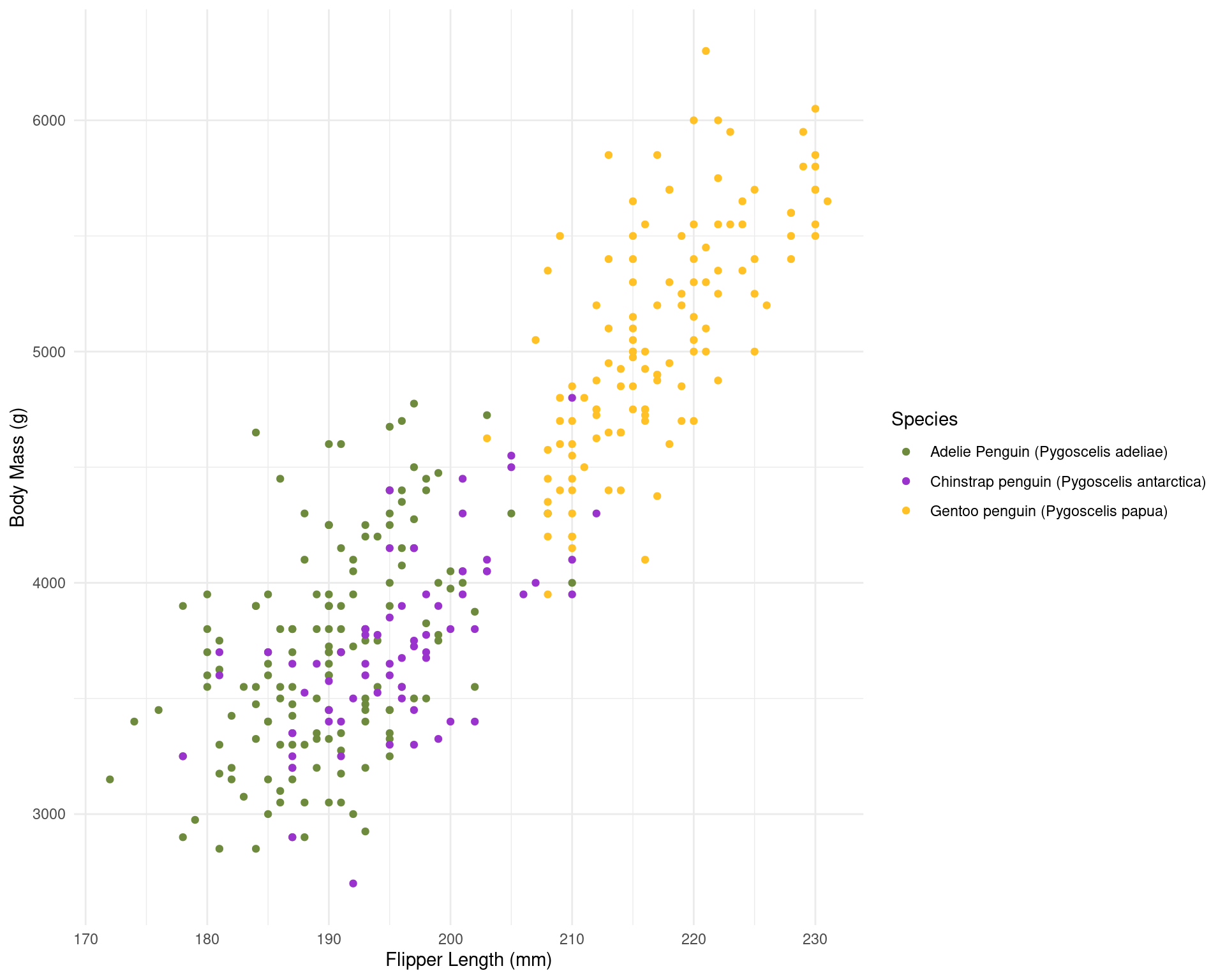
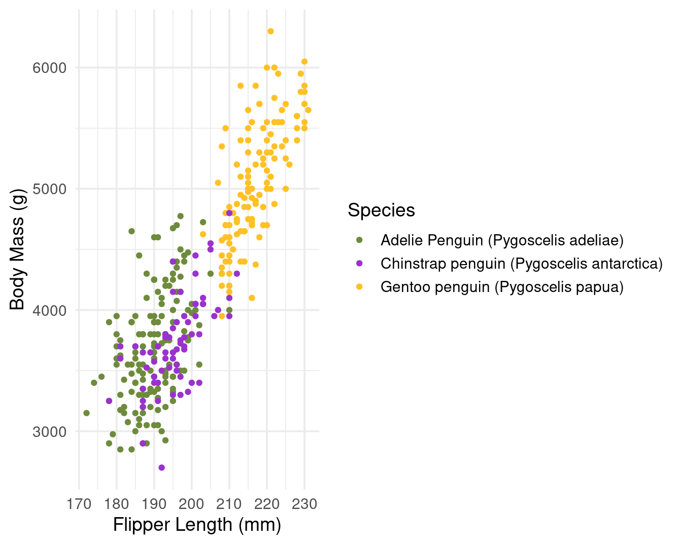
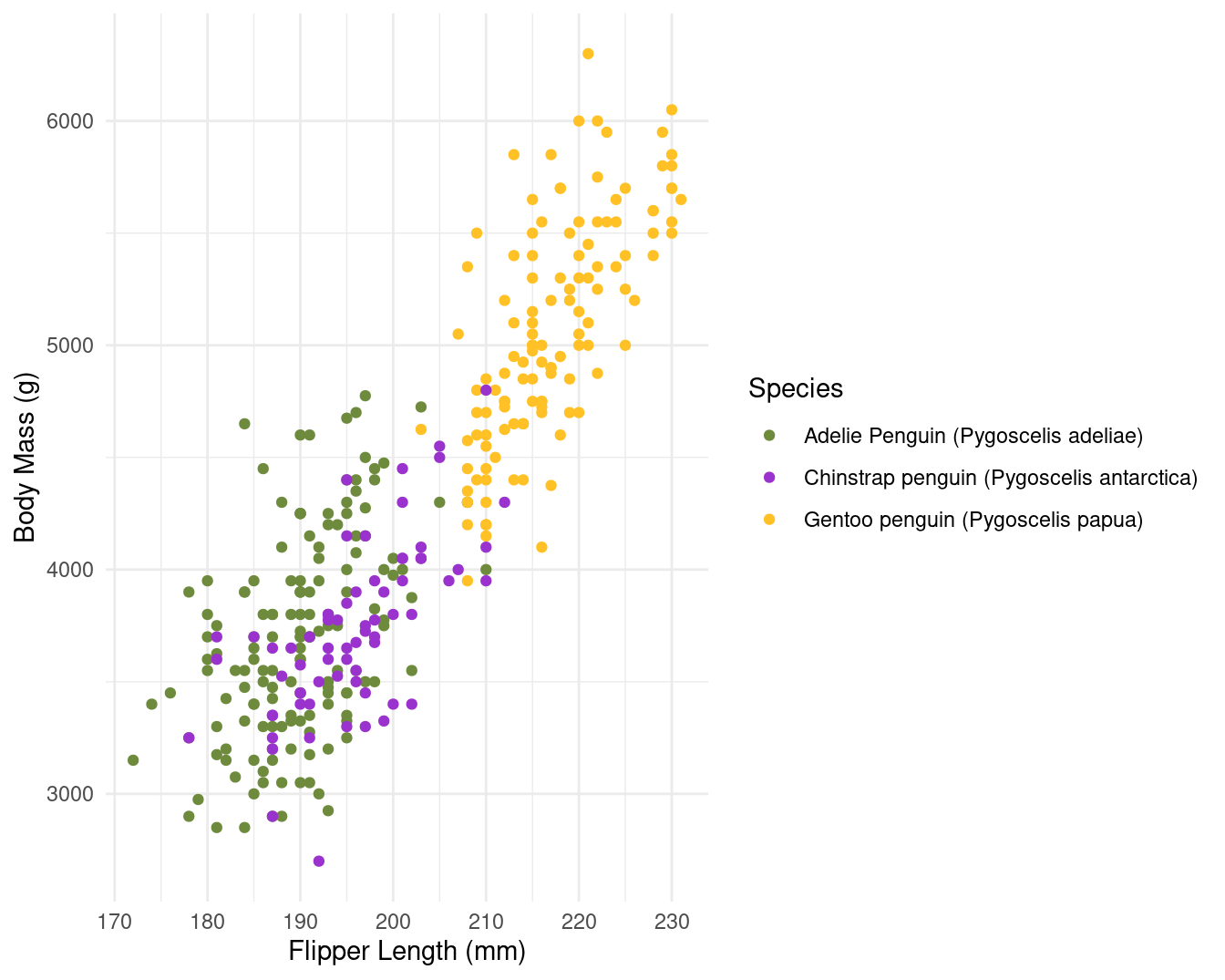
If you were making ggplot figures last session - you could source that script to put figures into your report
You will need to include a R chunk to print the figures - either by copying the code into a chunk, or assigning the plot to a named object in your R script and retrieving the name in your report R chunk.

```{r read-data}
#|include: false
# READ DATA ----

# Example replace with a script used for making ggplot figures if you have one
source("scripts/01_import_penguins_data.R")

```

```{r read-data}
#|echo: false

plot

```

Useful tips

Tip

The working directory for .qmd files is a little different to working with scripts.

With a .qmd file, the working directory is wherever the qmd file itself is saved.

For example if you have your .qmd file in a subfolder ~/outputfiles/markdown.qmd the code for read_csv(“data/data.csv”) within the markdown will look for a .csv file in a subfolder called data inside the ‘markdown’ folder and not the root project folder where the .RProj file lives.

So we have two options when using .qmd files

Don’t put the .qmd file in a subfolder and make sure it lives in the same directory as your .RProj file - that way relative filepaths are the same between R scripts and quarto files
Use the here package to describe file locations

Heuristic file paths with `here()`

The package here Müller (2025) and its function here() (here::here()), make it easy to tell R where to find and to save your files - in essence, it builds file paths. It becomes especially useful for dealing with the alternate filepaths generated by .qmd files, but can be used for exporting/importing any scripts, functions or data.

This is how here() works within an R project:

When the here package is first loaded within the R project, it places a small file called “.here” in the root folder of your R project as a “benchmark” or “anchor”
In your scripts, to reference a file in the R project’s sub-folders, you use the function here() to build the file path in relation to that anchor
To build the file path, write the names of folders beyond the root, within quotes, separated by commas, finally ending with the file name and file extension as shown below
here() file paths can be used for both importing and exporting

So when you use here() wrapped inside other functions for importing/exporting (like read_csv() or ggsave()) if you include here() you can still use the RProject location as the root directory when rendering Quarto files, even if your markdown is tidied away into a separate sub-folder.

This means your previous relative filepaths should be replaced with:

```{r, include=FALSE}
# PACKAGES ----
library(tidyverse)
library(here)

```

```{r}
#| include: false
# READ DATA ----

penguins <- read_csv(here("data", "penguins_raw.csv"))

head(penguins)

```

Warning

You might want start using the here() from now on to read in and export data from scripts. Make sure you are consistent in whether you use here() heuristic file paths or relative file paths across all .R and .qmd files in a project - otherwise you might encounter errors.

Hygiene tips

I recommend having three chunks at the top of any document

Global chunk options
All packages
Reading data


```{r setup , include=FALSE}
knitr::opts_chunk$set(echo = TRUE, 
                      fig.align = "center",
                      fig.width = 6,
                      fig.asp = 0.8,
                      out.width = "80%
                      )
                      
```

```{r library}
library(tidyverse)
```

```{r read-data}
source("scripts/02_visualisation_penguins.R")
```

Common knit issues

Any of these issues will cause the qmd document to fail to knit in its entirety. A failed knit is usually an easy fix, but needs you to READ the error message, and do a little detective work.

Duplication


```{r title-one}
```

```{r title-one}
```

Not the right order

plot(my_table)

my_table <- table(mtcars$cyl)

Forgotten trails

: Missing “,”, or “(”, “}”, or “’”

Path not taken

The qmd document is in a different location the .Rproj file causing issues with relative filepaths

Spolling

Incorrectly labelled chunk options
Incorrectly evaluated R code

Visual editor

RStudio comes with a pretty nifty Visual Markdown Editor which includes:

Spellcheck
Easy table & equation insertion
Easy citations and reference list building

You can switch between modes with a button push, try it out!

E.1 Background

How it works

Quarto parts

YAML Metadata

E.1.1 TASK: Can you edit the YAML in the Rmarkdown file in the markdown folder to have your name as author? Try changing the output to a different file type.

Code chunks

Text

Text emphasis

Titles and headings

Bullets and numbering

In-text code

Running code

E.2 Self contained Reports

E.2.1 TASK: Generate a self-contained report from data

ggplot

Size options for figures

Size of final figure in document

Static images

Tables

Markdown tables

gt()

Source files

Connecting scripts and reports

E.2.2 TASK: Create a separate R script for data import and quick cleaning save this and then source this into a new .qmd file.

Useful tips

Heuristic file paths with here()

Hygiene tips

Common knit issues

Duplication

Not the right order

Forgotten trails

Path not taken

Spolling

Visual editor

Further Reading, Guides and tips

Heuristic file paths with `here()`