Rows: 344
Columns: 17
$ studyName             <chr> "PAL0708", "PAL0708", "PAL0708", "PAL0708", "PAL…
$ `Sample Number`       <dbl> 1, 2, 3, 4, 5, 6, 7, 8, 9, 10, 11, 12, 13, 14, 1…
$ Species               <chr> "Adelie Penguin (Pygoscelis adeliae)", "Adelie P…
$ Region                <chr> "Anvers", "Anvers", "Anvers", "Anvers", "Anvers"…
$ Island                <chr> "Torgersen", "Torgersen", "Torgersen", "Torgerse…
$ Stage                 <chr> "Adult, 1 Egg Stage", "Adult, 1 Egg Stage", "Adu…
$ `Individual ID`       <chr> "N1A1", "N1A2", "N2A1", "N2A2", "N3A1", "N3A2", …
$ `Clutch Completion`   <chr> "Yes", "Yes", "Yes", "Yes", "Yes", "Yes", "No", …
$ `Date Egg`            <chr> "11/11/2007", "11/11/2007", "16/11/2007", "16/11…
$ `Culmen Length (mm)`  <dbl> 39.1, 39.5, 40.3, NA, 36.7, 39.3, 38.9, 39.2, 34…
$ `Culmen Depth (mm)`   <dbl> 18.7, 17.4, 18.0, NA, 19.3, 20.6, 17.8, 19.6, 18…
$ `Flipper Length (mm)` <dbl> 181, 186, 195, NA, 193, 190, 181, 195, 193, 190,…
$ `Body Mass (g)`       <dbl> 3750, 3800, 3250, NA, 3450, 3650, 3625, 4675, 34…
$ Sex                   <chr> "MALE", "FEMALE", "FEMALE", NA, "FEMALE", "MALE"…
$ `Delta 15 N (o/oo)`   <dbl> NA, 8.94956, 8.36821, NA, 8.76651, 8.66496, 9.18…
$ `Delta 13 C (o/oo)`   <dbl> NA, -24.69454, -25.33302, NA, -25.32426, -25.298…
$ Comments <chr> "Not enough blood for isotopes.", NA, NA, "Adult…7 Column classes & names
7.1 Learning Outcomes
This chapter explains how to check the class of each column and edit column names so that they are consistent and ready to use for analyses.
By the end of this section, you will be able to:
Identify the data class (type) of each column in a dataset.
Use functions to inspect and confirm column names and formats.
Apply
janitor::clean_names()to make variable names consistent and machine-readable.Rename columns manually using
dplyr::rename()when needed.
7.2 Column classes
Using glimpse() displays the class beside each column name (e.g. chr)
Using str() displays the class after the column name and before the number of rows (e.g. chr)
spc_tbl_ [344 × 17] (S3: spec_tbl_df/tbl_df/tbl/data.frame)
 $ studyName          : chr [1:344] "PAL0708" "PAL0708" "PAL0708" "PAL0708" ...
 $ Sample Number      : num [1:344] 1 2 3 4 5 6 7 8 9 10 ...
 $ Species            : chr [1:344] "Adelie Penguin (Pygoscelis adeliae)" "Adelie Penguin (Pygoscelis adeliae)" "Adelie Penguin (Pygoscelis adeliae)" "Adelie Penguin (Pygoscelis adeliae)" ...
 $ Region             : chr [1:344] "Anvers" "Anvers" "Anvers" "Anvers" ...
 $ Island             : chr [1:344] "Torgersen" "Torgersen" "Torgersen" "Torgersen" ...
 $ Stage              : chr [1:344] "Adult, 1 Egg Stage" "Adult, 1 Egg Stage" "Adult, 1 Egg Stage" "Adult, 1 Egg Stage" ...
 $ Individual ID      : chr [1:344] "N1A1" "N1A2" "N2A1" "N2A2" ...
 $ Clutch Completion  : chr [1:344] "Yes" "Yes" "Yes" "Yes" ...
 $ Date Egg           : chr [1:344] "11/11/2007" "11/11/2007" "16/11/2007" "16/11/2007" ...
 $ Culmen Length (mm) : num [1:344] 39.1 39.5 40.3 NA 36.7 39.3 38.9 39.2 34.1 42 ...
 $ Culmen Depth (mm)  : num [1:344] 18.7 17.4 18 NA 19.3 20.6 17.8 19.6 18.1 20.2 ...
 $ Flipper Length (mm): num [1:344] 181 186 195 NA 193 190 181 195 193 190 ...
 $ Body Mass (g)      : num [1:344] 3750 3800 3250 NA 3450 ...
 $ Sex                : chr [1:344] "MALE" "FEMALE" "FEMALE" NA ...
 $ Delta 15 N (o/oo)  : num [1:344] NA 8.95 8.37 NA 8.77 ...
 $ Delta 13 C (o/oo)  : num [1:344] NA -24.7 -25.3 NA -25.3 ...
 $ Comments           : chr [1:344] "Not enough blood for isotopes." NA NA "Adult not sampled." ...
 - attr(*, "spec")=
  .. cols(
  ..   studyName = col_character(),
  ..   `Sample Number` = col_double(),
  ..   Species = col_character(),
  ..   Region = col_character(),
  ..   Island = col_character(),
  ..   Stage = col_character(),
  ..   `Individual ID` = col_character(),
  ..   `Clutch Completion` = col_character(),
  ..   `Date Egg` = col_character(),
  ..   `Culmen Length (mm)` = col_double(),
  ..   `Culmen Depth (mm)` = col_double(),
  ..   `Flipper Length (mm)` = col_double(),
  ..   `Body Mass (g)` = col_double(),
  ..   Sex = col_character(),
  ..   `Delta 15 N (o/oo)` = col_double(),
  ..   `Delta 13 C (o/oo)` = col_double(),
  ..   Comments = col_character()
  .. )
 - attr(*, "problems")=<externalptr>
The skimr::skim() function groups columns by their type/class.
| Name | penguins_raw |
| Number of rows | 344 |
| Number of columns | 17 |
| _______________________ | |
| Column type frequency: | |
| character | 10 |
| numeric | 7 |
| ________________________ | |
| Group variables | None |
Variable type: character
| skim_variable | n_missing | complete_rate | min | max | empty | n_unique | whitespace |
|---|---|---|---|---|---|---|---|
| studyName | 0 | 1.00 | 7 | 7 | 0 | 3 | 0 |
| Species | 0 | 1.00 | 33 | 41 | 0 | 3 | 0 |
| Region | 0 | 1.00 | 6 | 6 | 0 | 1 | 0 |
| Island | 0 | 1.00 | 5 | 9 | 0 | 3 | 0 |
| Stage | 0 | 1.00 | 18 | 18 | 0 | 1 | 0 |
| Individual ID | 0 | 1.00 | 4 | 6 | 0 | 190 | 0 |
| Clutch Completion | 0 | 1.00 | 2 | 3 | 0 | 2 | 0 |
| Date Egg | 0 | 1.00 | 10 | 10 | 0 | 50 | 0 |
| Sex | 11 | 0.97 | 4 | 6 | 0 | 2 | 0 |
| Comments | 290 | 0.16 | 18 | 68 | 0 | 10 | 0 |
Variable type: numeric
| skim_variable | n_missing | complete_rate | mean | sd | p0 | p25 | p50 | p75 | p100 | hist |
|---|---|---|---|---|---|---|---|---|---|---|
| Sample Number | 0 | 1.00 | 63.15 | 40.43 | 1.00 | 29.00 | 58.00 | 95.25 | 152.00 | ▇▇▆▅▃ |
| Culmen Length (mm) | 2 | 0.99 | 43.92 | 5.46 | 32.10 | 39.23 | 44.45 | 48.50 | 59.60 | ▃▇▇▆▁ |
| Culmen Depth (mm) | 2 | 0.99 | 17.15 | 1.97 | 13.10 | 15.60 | 17.30 | 18.70 | 21.50 | ▅▅▇▇▂ |
| Flipper Length (mm) | 2 | 0.99 | 200.92 | 14.06 | 172.00 | 190.00 | 197.00 | 213.00 | 231.00 | ▂▇▃▅▂ |
| Body Mass (g) | 2 | 0.99 | 4201.75 | 801.95 | 2700.00 | 3550.00 | 4050.00 | 4750.00 | 6300.00 | ▃▇▆▃▂ |
| Delta 15 N (o/oo) | 14 | 0.96 | 8.73 | 0.55 | 7.63 | 8.30 | 8.65 | 9.17 | 10.03 | ▃▇▆▅▂ |
| Delta 13 C (o/oo) | 13 | 0.96 | -25.69 | 0.79 | -27.02 | -26.32 | -25.83 | -25.06 | -23.79 | ▆▇▅▅▂ |
If you are using a tibble, the class is also displayed below each column name when you view your data.
NoteData classes
From these data overviews we’ve learned:
Columns like
Species,Islandare strings of text (character)Columns like
Culmen Depth (mm)andFlipper Length (mm)are numbers with decimal points (double)
7.3 Column names
 [1] "studyName"           "Sample Number"       "Species"
 [4] "Region"              "Island"              "Stage"
 [7] "Individual ID"       "Clutch Completion"   "Date Egg"
[10] "Culmen Length (mm)"  "Culmen Depth (mm)"   "Flipper Length (mm)"
[13] "Body Mass (g)"       "Sex"                 "Delta 15 N (o/oo)"
[16] "Delta 13 C (o/oo)"   "Comments"
When we run colnames() we get the identities of each column in our dataframe
Study name: an identifier for the year in which sets of observations were made
Region: the area in which the observation was recorded
Island: the specific island where the observation was recorded
Stage: Denotes reproductive stage of the penguin
Individual ID: the unique ID of the individual
Clutch completion: if the study nest observed with a full clutch e.g. 2 eggs
Date egg: the date at which the study nest observed with 1 egg
Culmen length: length of the dorsal ridge of the bird’s bill (mm)
Culmen depth: depth of the dorsal ridge of the bird’s bill (mm)
Flipper Length: length of bird’s flipper (mm)
Body Mass: Bird’s mass in (g)
Sex: Denotes the sex of the bird
Delta 15N : the ratio of stable Nitrogen isotopes 15N:14N from blood sample
Delta 13C: the ratio of stable Carbon isotopes 13C:12C from blood sample
7.3.1 Problems:
Spaces and brackets make names awkward to reference.
R is case-sensitive — Mass ≠ mass.
You need backticks (```) around names with spaces or symbols.
Your turn
Identify two columns in penguins_raw that could cause errors if used without backticks:
7.3.1.1 Clean column names
Often we might want to change the names of our variables. They might be non-intuitive, or too long. Our data has a couple of issues:
Some of the names contain spaces
Some of the names have capitalised letters
Some of the names contain brackets
R is case-sensitive and also doesn’t like spaces or brackets in variable names, because of this we have been forced to use backticks `Sample Number` to prevent errors when using these column names.
ImportantName consistency
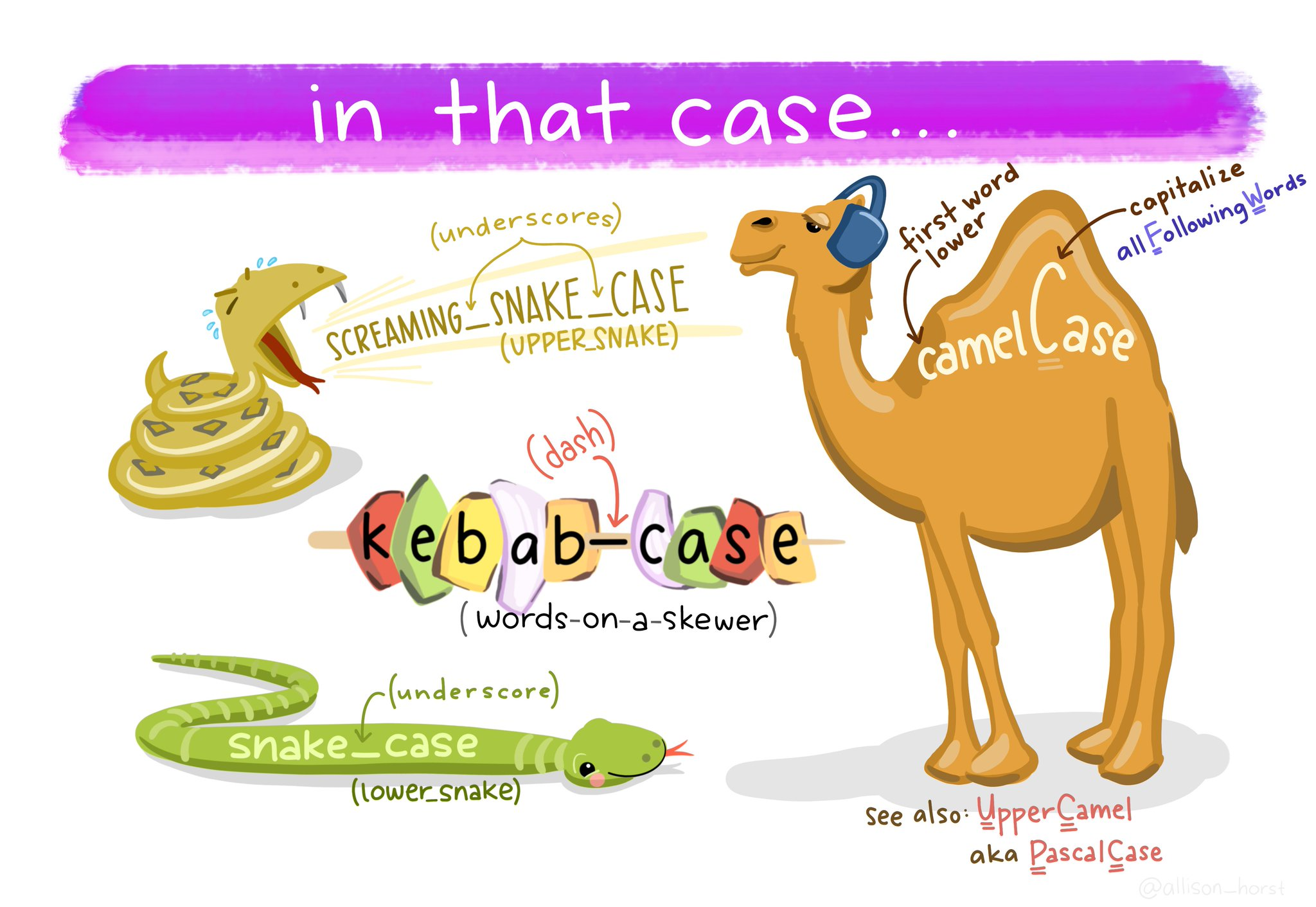
Column names should use consistent naming conventions. R is case sensitive, so two names with the same letters but different capitalisations are considered different names (e.g. event vs. Event). Using a naming convention which is both human- and machine-readable (e.g. camel case, snake case), and being consistent in your usage of it, makes it less likely that you will make these sorts of errors.
-
Snake case uses lowercase letters only, with words separated by an underscore _ (e.g.
scientific_name,data_resource_name,event_date).
One of the most useful column name cleaning functions is janitor::clean_names() from the janitor package Firke (2024). This function will make all of your column names consistent, based on your preferred naming convention (defaults to snake case).
# CLEAN DATA ----

# clean all variable names to snake_case
# using the clean_names function from the janitor package
# note we are using assign <-
# to overwrite the old version of penguins
# with a version that has updated names
# this changes the data in our R workspace
# but NOT the original csv file

# clean the column names
# assign to new R object
penguins_clean_names <- janitor::clean_names(penguins_raw)

# quickly check the new variable names
colnames(penguins_clean_names)
[1] "study_name" "sample_number" "species"
[4] "region" "island" "stage"
[7] "individual_id" "clutch_completion" "date_egg"
[10] "culmen_length_mm" "culmen_depth_mm" "flipper_length_mm"
[13] "body_mass_g" "sex" "delta_15_n_o_oo"
[16] "delta_13_c_o_oo" "comments" 7.3.1.2 Rename columns (manually)
The clean_names function quickly converts all variable names into snake caseSnake case is a naming convention in computing that uses underscores to replace spaces between words, and writes words in lowercase. It’s commonly used for variable names, filenames, and database table and column names.. The N and C blood isotope ratio names are still quite long though, so let’s clean those with dplyr::rename() where “new_name” = “old_name”.
7.4 Save Cleaned Data
Saving as .RDS ensures you can load the cleaned version quickly next time.