23 Causal models

# Required packages
library(here)
library(tidyverse)
library(GGally)
library(skimr)
library(colorspace)
library(ggridges)
library(performance)
library(patchwork)
library(ggdag)

23.1 The data

We are introduced to the fruitfly dataset (Partridge and Farquhar (1981))[https://nature.com/articles/294580a0]. From our understanding of sexual selection and reproductive biology in fruit flies, we know there is a well established ‘cost’ to reproduction in terms of reduced longevity for female fruitflies. The data from this experiment is designed to test whether increased sexual activity affects the lifespan of male fruitflies.

The flies used were an outbred stock, sexual activity was manipulated by supplying males with either new virgin females each day, previously mated females (Inseminated, so remating rates are lower), or provide no females at all (Control). For virgin and inseminated treatments, males were provided either a single female, or a group of females (8). All groups were otherwise treated identically.

partners: number of female companions(virgin = 1 or 8, inseminated = 1 or 8, control = 0)
type: type of female companion (virgin, inseminated, control(partners = 0))
longevity: lifespan in days
thorax: length of thorax in micrometres (a proxy for body size)
sleep: percentage of the day spent sleeping

dros_clean <- read_csv(here::here("data","clean", "fruitfly.csv"))

Factors

What order will R organise the three type categories?

In linear models, when we test groups one group will always be the Intercept (reference group). By default this will be alphabetical unless the levels have an order specified by making them a factor

dros_clean |> 
  mutate(type = factor(type, 
                       levels = c("Control", 
                                  "Inseminated", 
                                  "Virgin")))

23.1.1 Questions

Think about causal relationships. Which variables might cause which others?

Write down some ideas:

Does mating status of the female affect male longevity (via changes in sexual activity)?
Does body size affect longevity directly?
Does body size affect longevity via change in mating activity?
Does sleep affect longevity?
Does female mating status or the number of females affect male sleep?

23.2 Checking the data

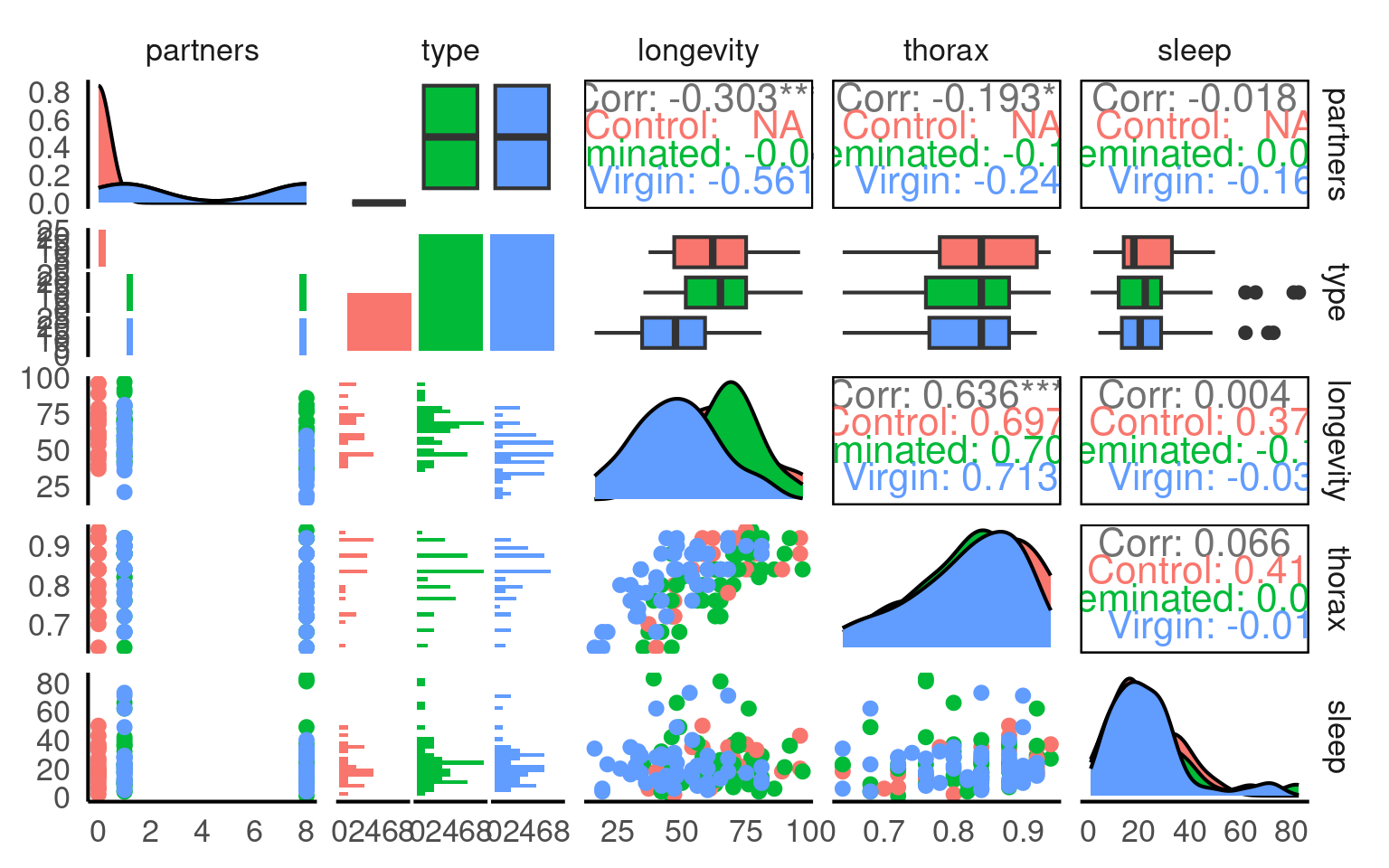
A quick intro to a general overview:

This is a full two-by-two plot of the entire dataset, but you should try and follow this up with some specific plots.

GGally::ggpairs(dros_clean,
                ggplot2::aes(colour = type)) # separates geoms by type a key variable in our hypotheses

Your turn

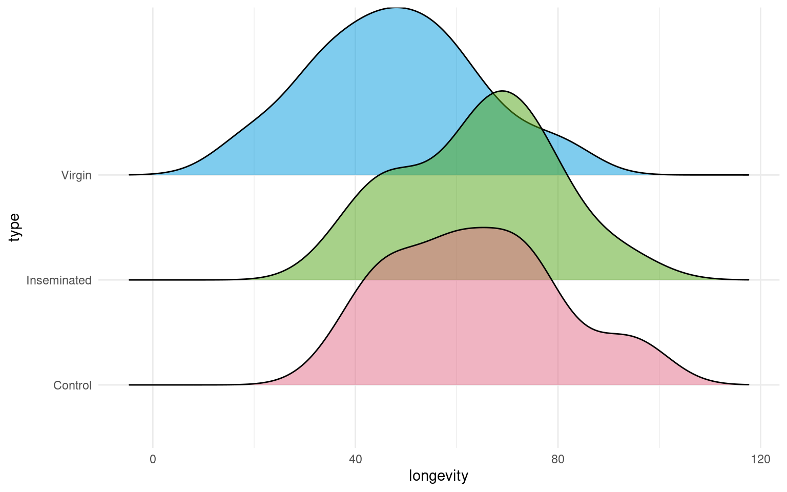
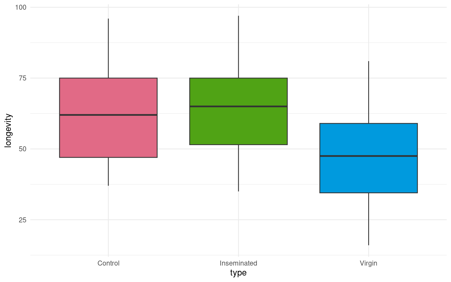
Make a Boxplot / Density distribution of longevity split by the female type with which males have been paired

dros_clean |> 
  ggplot(aes(x = longevity, y = type, fill = type))+
  geom_density_ridges(alpha = 0.5)+
  scale_fill_discrete_qualitative() +
  theme_minimal()+
  theme(legend.position = "none")

dros_clean |> 
  ggplot(aes(x = type, y = longevity, fill = type))+
  geom_boxplot()+
  scale_fill_discrete_qualitative() +
  theme_minimal()+
  theme(legend.position = "none")

23.3 The Causal Question

In this section, we explore how to construct a statistical model to analyse biological data. Specifically, we will build a linear model to examine our main question of whether female mating type affects male longevity in Drosophila melanogaster .

In order to do this we need to confirm our proposed relationships between variables - and produce our first use directed acyclic graphA diagram showing assumed causal relationships; arrows indicate cause, and loops are not allowed. (DAGs) to make better decisions about statistical modelling in biological research.

Your turn

Write out your proposed relationships:

These are not interaction effects these are proposals about which variables cause changes in the others

Mating status → sleep
Mating status → longevity
Mating status → Number of partners
Number of partners → sleep
Number of partners → longevity
Sleep → longevity
Thorax → longevity

Can you identify which of these are an outcomeThe variable affected by the exposure., exposureA variable we are interested in intervening on.?

library(ggdag)

fly_dag <- dagify(
  longevity ~ type + sleep + thorax + partners,
  sleep ~ type + partners,
  partners ~ type,
  exposure = "type",
  outcome = "longevity"
)

ggdag_status(fly_dag, layout = "circle") +
    theme_dag() +
    ggtitle("Exposure and Outcome Labels")

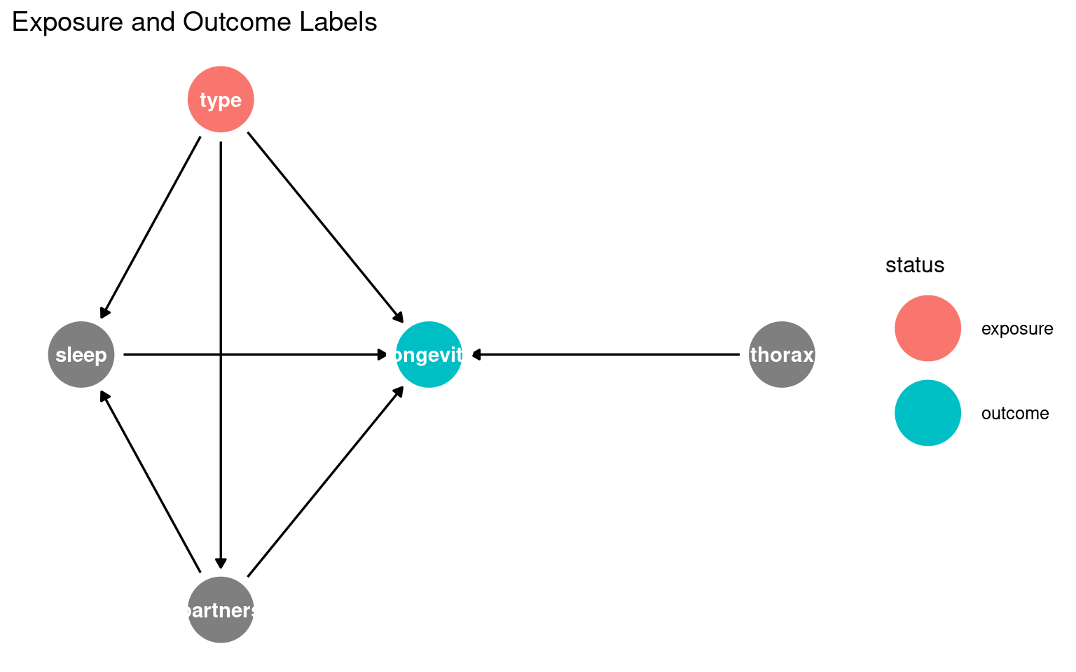
23.3.1 What this shows:

Nodes = variables
Arrows = causal relationships
type = exposure
longevity = outcome
You can start recognising candidate mediators (sleep, partners) and possible confounders (thorax) visually.

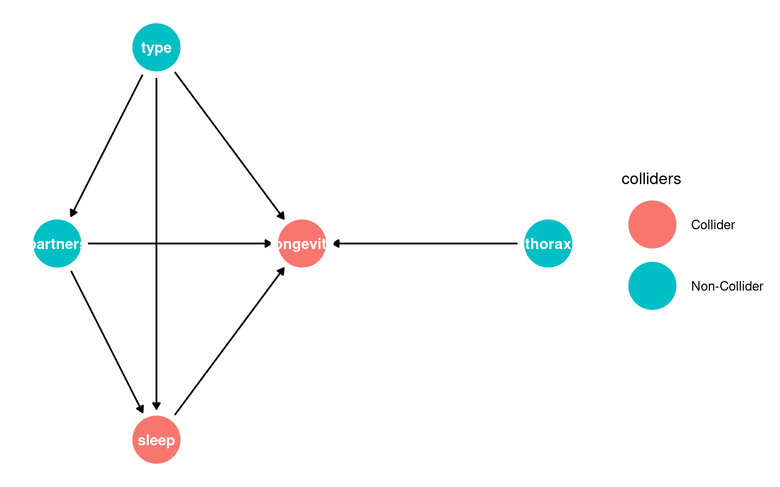
23.3.2 Identifying colliders

Next it is important to whether any variables migh act as a potential colliderA variable influenced by two or more other variables; adjusting for it can create spurious associations..
A collider looks like this X → Z ← Y, where Z is the collider being influenced by both X and Y.

Conditioning on colliders opens non-causal paths and can create spurious associations. This is a common source of bias.

# Find colliders
ggdag_collider(fly_dag)+ theme_dag()

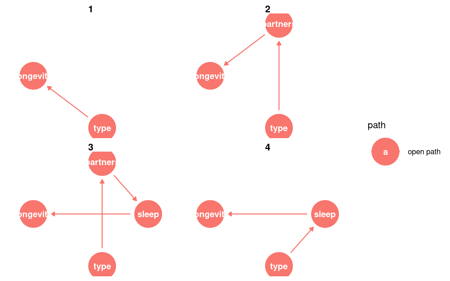
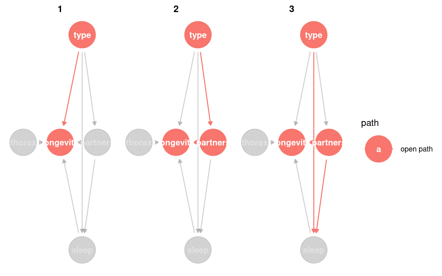
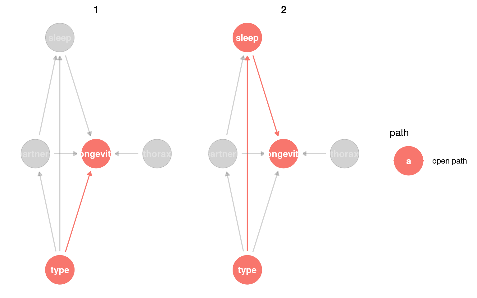
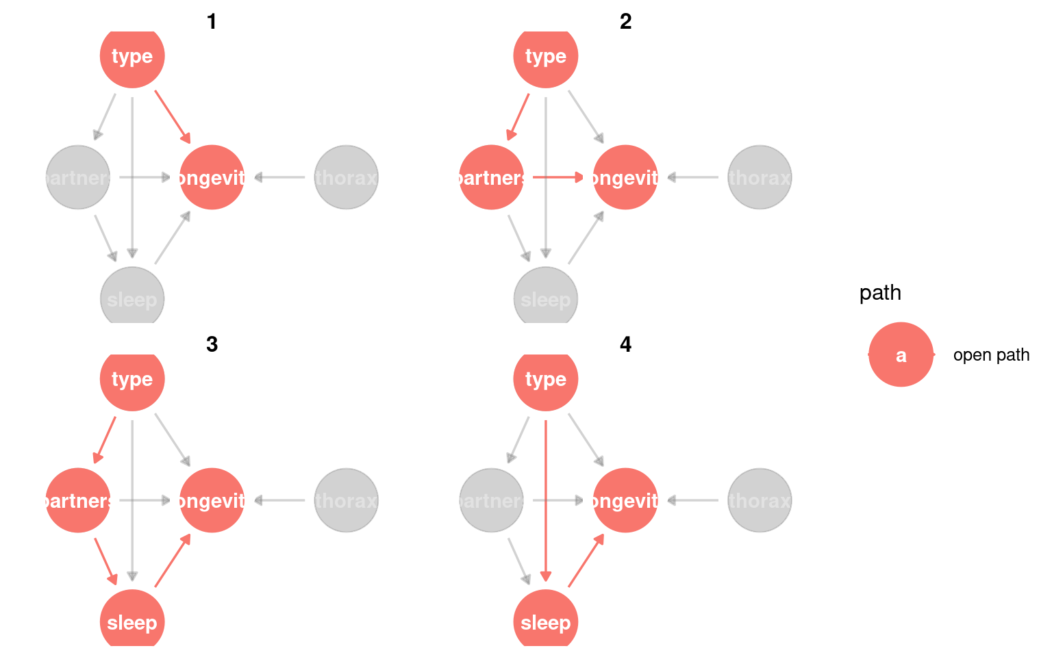
23.3.3 Identifying causal paths

This helps us identify all of the routes from exposure to outcome. Any variable on a path between the two can be considered a mediatorA variable on the causal path from exposure to outcome; it transmits part of the effect.

Variables that lie on a directed path and are downstream of the exposure are mediators, because they transmit part of the causal effect.

We could also look for whether any variable is a confounderA variable that affects both the exposure and the outcome, potentially creating a false association. - this would be any variable that causes changes to type and longevity.

Variables that appear on paths but are upstream of the exposure are not mediators; they are potential confounders.

# Examine all paths
ggdag_paths(fly_dag, 
            from = "type", 
            to = "longevity")+
  theme_dag()

Important

Including a mediator will mean the “total effect” of the exposure cannot be estimated, only the “direct effect”.

Including a collider will bias the model as it opens a “non-causal” path.

23.3.4 Check adjustment sets

Here we can identify the variables that “must be conditioned on” in order to estimate the total causal effect on outcome.

# Get adjustment sets
ggdag_adjustment_set(fly_dag)+ theme_dag()

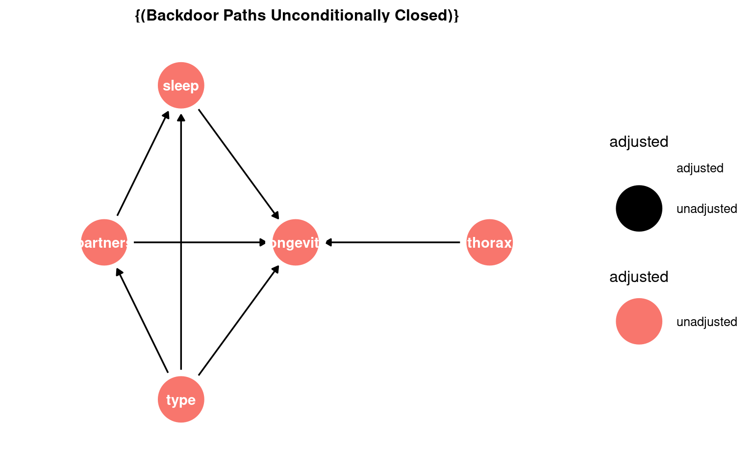
In this DAG there are no adjustments required:

dagitty::adjustmentSets(fly_dag,
               exposure = "type",
               outcome  = "longevity")

{}

ggdag_paths(fly_dag, adjust_for = "sleep", shadow = TRUE)+ theme_dag()

ggdag_paths(fly_dag, adjust_for = "partners", shadow = TRUE)+ theme_dag()

ggdag_paths(fly_dag, adjust_for = "thorax", shadow = TRUE)+ theme_dag()

23.4 Building models

Using the lm() function in R, we fit a model to our cleaned dataset, and generate a summary of the results. This approach allows us to assess the significance of each predictor and interpret how these factors influence longevity. By the end of this section, you will understand how to structure a model, choose appropriate variables, and interpret statistical outputs.

If we want the direct and total effect of type we have seen that we do not need to include any other adjustment variables:

# Total effect
model_total <- lm(longevity ~ type, data = dros_clean)

Our DAG also included body size (thorax) as a causal variable on longevity that is not part of the same causal paths as type. We can include this variable if we want to increase the variance explained, and precision of our estimates.

# Total effect + precision
model_total_precise <- lm(longevity ~ type + thorax, data = dros_clean)

This model should be used if we wish to estimate only the direct effect of type (i.e. only the effect which is not mediated by sleep and partners).

model_direct <- lm(longevity ~ type + thorax + sleep + partners, data = dros_clean)

summary(model_total)


Call:
lm(formula = longevity ~ type, data = dros_clean)

Residuals:
   Min     1Q Median     3Q    Max 
-31.74 -13.74   0.26  11.44  33.26 

Coefficients:
                Estimate Std. Error t value Pr(>|t|)    
(Intercept)       63.560      3.158  20.130  < 2e-16 ***
typeInseminated    0.520      3.867   0.134    0.893    
typeVirgin       -15.820      3.867  -4.091 7.75e-05 ***
---
Signif. codes:  0 '***' 0.001 '**' 0.01 '*' 0.05 '.' 0.1 ' ' 1

Residual standard error: 15.79 on 122 degrees of freedom
Multiple R-squared:  0.2051,    Adjusted R-squared:  0.1921 
F-statistic: 15.74 on 2 and 122 DF,  p-value: 8.305e-07

broom::tidy(model_total)

term	estimate	std.error	statistic	p.value
(Intercept)	63.56	3.157477	20.1299982	0.0000000
typeInseminated	0.52	3.867103	0.1344676	0.8932544
typeVirgin	-15.82	3.867103	-4.0909173	0.0000775

23.5 Confidence intervals

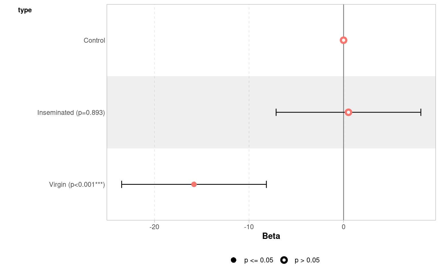
When we produce a model fit - it is useful to think in terms of confidence intervals and estimate differences rather than just p-values.

A 95% confidence interval give us our confidence in having captured the true difference between groups at p = 0.05

broom::tidy(model_total, conf.int = T)

term	estimate	std.error	statistic	p.value	conf.low	conf.high
(Intercept)	63.56	3.157477	20.1299982	0.0000000	57.309460	69.810541
typeInseminated	0.52	3.867103	0.1344676	0.8932544	-7.135317	8.175317
typeVirgin	-15.82	3.867103	-4.0909173	0.0000775	-23.475317	-8.164683

GGally::ggcoef_model(model_total)

Term	Estimate	95% CI	Interpretation
(Intercept)	63.6	(57.3, 69.8)	Baseline longevity — flies in the reference group (mated males) live about 64 days on average. We are 95% confident the true mean lies between 57 and 70 days.
typeInseminated	0.52	(−7.1, 8.2)	Flies with inseminated partners live about 0.5 days longer than the reference group, but the 95% CI spans both negative and positive values — from −7 to +8 days — indicating no clear difference.
typeVirgin	−15.8	(−23.5, −8.2)	Flies paired with virgin partners live roughly 16 days shorter on average. The 95% CI (−23.5 to −8.2) does not include zero, within our confidence intervals we know that the true difference is at least 8.2 days

23.6 Precison model

In a basic linear model, we often start by comparing group means — for example:

\[ \text{longevity}_i = \beta_0 + \beta_1 \, \text{type}_i + \varepsilon_i \]

This model assumes that differences in longevity are entirely due to type (e.g., mating partner).

But in real data, other variables may also influence the outcome — for example, body size might affect how long flies live.

If mean body size happens to vary slightly between groups, failing to include it could confound our estimate of the effect of type.

By adding it as a covariate, we adjust for this additional source of variation:

\[ \text{longevity}_i = \beta_0 + \beta_1 \, \text{type}_i + \beta_2 \, \text{thorax}_i + \varepsilon_i \]

23.6.1 Interpretation

The coefficient 𝛽1 represents the effect of mating type, after adjusting for body size.
The coefficient 𝛽2 represents how longevity changes with body size, holding type constant.
Including covariates often reduces residual variation and improves model fit.

model_total_precise <- lm(longevity ~ type + thorax, data = dros_clean)

Your turn

Fit the updated model
What does it say about the effect of body size (thorax) on longevity?
What is the adjusted effect of the type on longevity?

summary(model_total_precise)


Call:
lm(formula = longevity ~ type + thorax, data = dros_clean)

Residuals:
    Min      1Q  Median      3Q     Max 
-27.330  -6.803  -2.531   7.143  29.415 

Coefficients:
                Estimate Std. Error t value Pr(>|t|)    
(Intercept)      -56.521     11.149  -5.069 1.45e-06 ***
typeInseminated    3.450      2.759   1.250    0.214    
typeVirgin       -13.349      2.756  -4.845 3.80e-06 ***
thorax           143.638     13.064  10.995  < 2e-16 ***
---
Signif. codes:  0 '***' 0.001 '**' 0.01 '*' 0.05 '.' 0.1 ' ' 1

Residual standard error: 11.21 on 121 degrees of freedom
Multiple R-squared:  0.6024,    Adjusted R-squared:  0.5925 
F-statistic:  61.1 on 3 and 121 DF,  p-value: < 2.2e-16

When we use continuous predictors, the intercept becomes the expected value of our outcome (longevity), when all predictors are 0. This can make the intercept an unrealistic value.

One way around this is to “center” the continuous predictors - so that 0 now becomes the mean value of the predictor

dros_clean$thorax_c <- scale(dros_clean$thorax, scale = FALSE)

model_total_precise_c <- lm(longevity ~ type + thorax_c, data = dros_clean)

summary(model_total_precise_c)


Call:
lm(formula = longevity ~ type + thorax_c, data = dros_clean)

Residuals:
    Min      1Q  Median      3Q     Max 
-27.330  -6.803  -2.531   7.143  29.415 

Coefficients:
                Estimate Std. Error t value Pr(>|t|)    
(Intercept)       61.400      2.251  27.277  < 2e-16 ***
typeInseminated    3.450      2.759   1.250    0.214    
typeVirgin       -13.349      2.756  -4.845  3.8e-06 ***
thorax_c         143.638     13.064  10.995  < 2e-16 ***
---
Signif. codes:  0 '***' 0.001 '**' 0.01 '*' 0.05 '.' 0.1 ' ' 1

Residual standard error: 11.21 on 121 degrees of freedom
Multiple R-squared:  0.6024,    Adjusted R-squared:  0.5925 
F-statistic:  61.1 on 3 and 121 DF,  p-value: < 2.2e-16

23.7 Compare the models

Compare to the simpler model:

anova(model_total, model_total_precise_c)

Res.Df	RSS	Df	Sum of Sq	F	Pr(>F)
122	30407.46	NA	NA	NA	NA
121	15210.85	1	15196.61	120.8868	0

The ANOVA tests whether adding body_size significantly improves the model.

23.8 Causal DAG and `ggdag` Checklist

23.8.0.1 1. Define the causal question

Clearly specify the exposure and outcome
State the causal estimand:
- Total effect, or
- Direct effect (and through which pathways)

23.8.0.2 2. Draw and inspect the DAG

Encode substantive causal assumptions as arrows
Ensure arrow directions reflect causal ordering, not statistical association
Check that all relevant common causes are represented

23.8.0.3 3. Identify causal paths

Examine directed paths from exposure to outcome
Classify variables by their position relative to the exposure:
- Downstream of exposure → candidate mediators
- Upstream of exposure → candidate confounders
Remember: being on a path is necessary but not sufficient for mediation

23.8.0.4 4. Identify colliders

Locate nodes where arrows meet head-to-head (X → Z ← Y)
Do not condition on colliders, including outcome colliders

23.8.0.5 5. Check for confounding

Use adjustmentSets() to identify sufficient adjustment sets
Confirm whether confounding exists for the chosen estimand
Note: adjustment sets indicate how to adjust, not which variables are confounders

23.8.0.6 6. Decide what to include in the model

Include confounders (if present) to remove bias
Exclude mediators when estimating total effects
Include mediators only when estimating direct effects, with assumptions stated
Exclude colliders
Variables that affect only the outcome may be included for precision, not bias control

23.8.0.7 7. Fit and interpret the model

Fit the statistical model consistent with the estimand
Interpret coefficients only with respect to the causal question posed
Avoid interpreting “adjusted” coefficients as causal without DAG justification

23.8.0.8 Core principle

Draw the DAG → identify paths → classify variables → choose the estimand → then model.

23.1 The data

23.1.1 Questions

23.2 Checking the data

23.3 The Causal Question

23.3.1 What this shows:

23.3.2 Identifying colliders

23.3.3 Identifying causal paths

23.3.4 Check adjustment sets

23.4 Building models

23.5 Confidence intervals

23.6 Precison model

23.6.1 Interpretation

23.7 Compare the models

23.8 Causal DAG and ggdag Checklist

23.8.0.1 1. Define the causal question

23.8.0.2 2. Draw and inspect the DAG

23.8.0.3 3. Identify causal paths

23.8.0.4 4. Identify colliders

23.8.0.5 5. Check for confounding

23.8.0.6 6. Decide what to include in the model

23.8.0.7 7. Fit and interpret the model

23.8.0.8 Core principle

23.8 Causal DAG and `ggdag` Checklist