1  R Basics

R is a programming language and environment for statistical computing and graphics. RStudio is an Integrated Development Environment (IDE) that makes using R easier by providing a user-friendly interface with helpful features (like a script editor, console, environment viewer, etc.). In other words, you write and run R code, and RStudio helps you organize and execute that code more conveniently. For this course, we can use RStudio (via Posit Cloud) to write and run R code, but remember that R and RStudio are two separate pieces of software – R is the engine under the hood, and RStudio is the dashboard and controls. Both R and RStudio may have their own updates, so keep an eye on updating them separately when working on your personal computer.

Tip: R and RStudio are free to download. You can install R from the CRAN website (Comprehensive R Archive Network) and RStudio from the Posit (formerly RStudio) website. In our classroom environment on Posit Cloud, these are already set up for you.

1.1 Your first R command

Let’s try some simple calculations in R to get a feel for it. You can use R as a calculator:

# Addition
10 + 20

• What answer did you get?

30

Note

The first line shows the request you made to R, the next line is R’s response

You didn’t type the > symbol: that’s just the R command prompt and isn’t part of the actual command.

Your turn

Here are some other basic arithmetic examples to try:

13 - 10    # Subtraction
4 * 6      # Multiplication
12 / 3     # Division
5^4        # Exponentiation (5 to the power of 4)

1.1.1 Perform some combos

You can combine operations, and R will follow the standard order of operations (BODMAS/BIDMAS rules: Brackets/Parentheses, Orders/Exponents, Division and Multiplication, Addition and Subtraction). For example:

3^2 - 5/2      # R will do 3^2 = 9, then 9 - (5/2) = 9 - 2.5

(3^2 - 5) / 2  # R will do the part in parentheses first: (9 - 5) = 4, then 4/2 = 2

Warning

Be careful with parentheses to ensure calculations happen in the order you intend. If you omit parentheses, R might give a different result than you expect.

1.1.2 Use R interactively:

Don’t be afraid to experiment in the console. R is read-evaluate-print by nature: you type an expression, R evaluates it, and prints the result. If you type an incomplete expression, R will show a + continuation prompt, meaning it’s waiting for the rest of your input. For instance, if you type 10 + and press Enter, the console will show:

> 10 +
+ 

That + indicates R expects more input (it knows the command isn’t complete).

• If you realize you made a mistake and want to cancel, press Esc to break out and get back to the > prompt.

• Otherwise, you can continue the command (type 20 and hit Enter) to complete it:

Your turn

Write an incomplete line of code - then either finish it or escape the line of code

> 10 +
+ 20

[1] 30

1.1.3 Comparison operators

R can also compare values. These expressions return logical values: TRUE or FALSE.

5 > 3

5 == 3

5 != 3

Note

Here, == means “equal to”. A single = is not used for comparison in R.

Your turn

How would you write the code to check that 7 is less than or equal to 5?

7 <= 5

[1] FALSE

1.2 Objects and assignment

R is object-based. This means you usually store results so you can reuse them later.

x <- 10 + 20

Here we created a variable named x and assigned it the result of 10 + 20 (which is 30). This does not print 30 to the console because the result was instead stored in x.

If you want to see the value, you can simply type x in the console and press Enter:

x 

Typing the name of a variable and hitting Enter will print its value (this is called auto-printing). Alternatively, you could use the explicit print(x) function with the same result. In interactive use, auto-printing by typing the name is convenient; in scripts or functions, you might use print() to display interim results.

You can use variables in calculations just like numbers. Continuing the example, since x is 30:

x * 2    # This will give 60, since x is 30
x + 5    # This will give 35

[1] 60
[1] 35

You can also assign the results of these calculations to new variables:

y <- x * 2       # y will be 60
z <- x + y + 5   # z will be 30 + 60 + 5 = 95

After these assignments, you will see x, y, and z listed in RStudio’s Environment pane with their values. At any time, you can inspect a variable’s value by printing it (as shown above).

Note

The arrow <- assigns the value on the right to the name on the left. If you assign a new value to the same name, the old value is overwritten.

x <- 100

1.3 Vectors

A vector is the simplest data structure in R. It is a collection of values of the same type.

nums  <- c(1, 2, 3)
chars <- c("a", "b", "c")

Note

The function c() stands for “combine”.

1.3.1 Sequences

R can generate sequences easily

1:5

[1] 1 2 3 4 5

1.3.2 Indexing

R starts counting from 1, not 0:

nums[1]

[1] 1

nums[c(1, 3)]

[1] 1 3

1.3.3 Logical subsetting

You can select values from within a vector that meet a condition:

scores <- c(85, 92, 76, 81, 90)

# retrieve only those scores greater than 80.
scores[scores > 80]

[1] 85 92 81 90

Your turn

How would you write the code that retrieves only values less than or equal to 81?

scores[scores <= 81]

[1] 76 81

1.3.4 Vectorised operations

Most operations in R work element-by-element.

nums * 2

[1] 2 4 6

nums + c(10, 20, 30)

[1] 11 22 33

Your turn

1. Create a vector called ages containing five ages.

ages <- c(12, 24, 37, 29, 8)

2. Extract the second and fourth values.

ages[c(2,4)]

[1] 24 29

3. Select only the ages greater than 30.

ages[ages>30]

[1] 37

4. Add 5 to every value in ages.

ages+5

[1] 17 29 42 34 13

1.4 Variable naming rules and tips

courtesy of Allison Horst

• Use meaningful names: It’s often better to use descriptive names for variables (e.g., total_sales instead of x or var1) so that the code is self-explanatory. This helps you (and others) understand the code later.

• Be concise: While names should be meaningful, overly long names can be cumbersome. Try to strike a balance (e.g., response_time is easier to handle than the_response_time_of_the_subject).

• No spaces or special characters: Variable names cannot contain spaces. They must start with a letter or dot (.) or underscore (_), and the remaining characters can be letters, numbers, dots, or underscores. For example, currentTemperature or current_temperature are valid names, but current temperature (with a space) is not. Also, avoid using symbols like +, -, * in names.

• Case sensitivity: R is case-sensitive. This means Variable, variable, and VARIABLE would be three different names. Be consistent in your naming to avoid confusion.

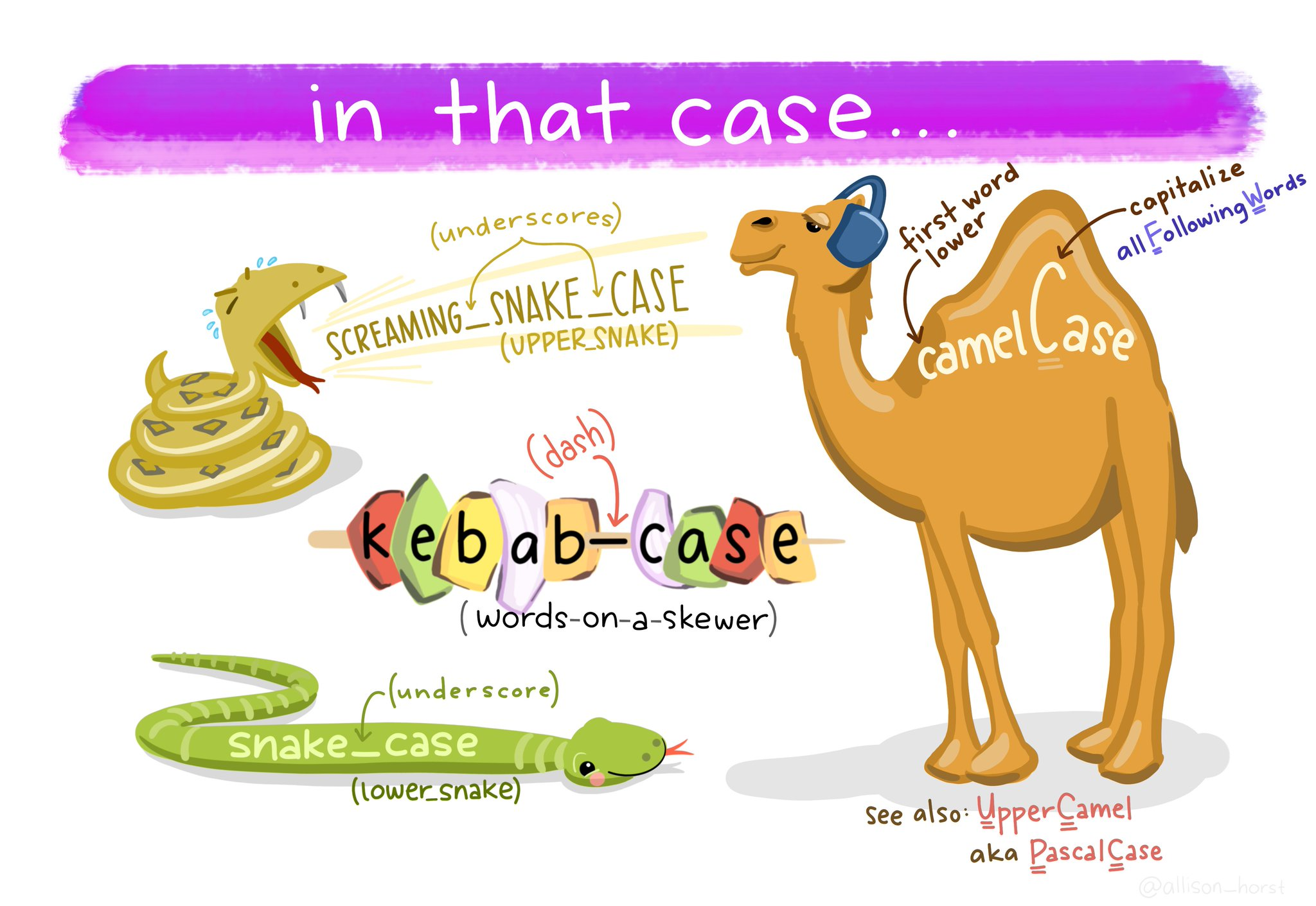
• Recommended conventions: Many R programmers use either snake_case or camelCase for multi-word names. Snake case uses underscores (e.g., total_cost), while camel case capitalizes each word after the first (e.g., totalCost). Choose one style and stick with it.

Warning

Avoid naming variables after existing functions or constants in R (like mean, data, T, c, etc.) because that can lead to confusion or errors. For instance, if you do mean <- 5, you won’t be able to use the mean() function until you restart R or remove that variable.

1.5 Dataframes and Tibbles

A data frame is a table. Each row represents an observation; each column represents a variable.

survey <- data.frame(
  "index" = c(1, 2, 3, 4, 5),
  "sex" = c("m", "m", "m", "f", "f"),
  "age" = c(99, 46, 23, 54, 23)
  )

This makes a data frame survey with 5 rows and 3 columns: index, sex, and age. If you print survey, you’ll see something like:

survey

index	sex	age
1	m	99
2	m	46
3	m	23
4	f	54
5	f	23

Each column is a vector: survey$index is the vector 1,2,3,4,5; survey$sex is c(“m”,“m”,“m”,“f”,“f”); survey$age is c(99,46,23,54,23).

Because each column is a vector, they all must be the same length (here length 5) – which they are.

1.5.1 Accessing columns

survey$age

[1] 99 46 23 54 23

survey[["age"]]

[1] 99 46 23 54 23

Both return the same column

1.5.2 Subsetting rows and columns

survey[1:3, c("sex", "age")]

sex	age
m	99
m	46
m	23

1.5.3 Adding a column

survey$follow_up <- c(TRUE, FALSE, TRUE, FALSE, FALSE)

survey

index	sex	age	follow_up
1	m	99	TRUE
2	m	46	FALSE
3	m	23	TRUE
4	f	54	FALSE
5	f	23	FALSE

1.5.4 Tibbles

Tibbles are a modern version of data frames with safer defaults and clearer printing.

library(tibble)

survey_tibble <- tibble(
  "index" = c(1, 2, 3, 4, 5),
  "sex" = c("m", "m", "m", "f", "f"),
  "age" = c(99, 46, 23, 54, 23)
  )

For most beginner tasks, data frames and tibbles can be treated as interchangeable.

If you print survey_tibble, you’ll get an output like:

survey_tibble

index	sex	age
1	m	99
2	m	46
3	m	23
4	f	54
5	f	23

1.6 Functions

Functions are the tools of R. Each one helps us to do a different task.

Functions perform specific tasks. You call a function by writing its name followed by parentheses ().

round(x, digits = 0)

This means round() takes an argument x (the number or vector to round) and an argument digits (how many decimal places to round to, which defaults to 0 if not specified).

round(x = 2.432678, digits = 2)

[1] 2.43

Arguments can be supplied by position or by name:

round(2.432678, 2)

[1] 2.43

round(digits = 2, x = 2.436)

[1] 2.44

1.6.1 Help

Getting help for functions: If you’re not sure how to use a function or what arguments it takes, use R’s help system:

• ?function_name (e.g., ?round) will bring up the help page for that function.

• The help page will usually show the usage, a description of each argument, details, examples, and more.

• You can also search for functions by keyword using ??keyword or help("keyword"). For example, ??rounding might show all help pages that mention rounding.

1.7 Packages

One of the biggest strengths of R is its rich ecosystem of packages. A package is a bundle of functions, data, and documentation, developed by the community, that extends R’s capabilities. Base R comes with a standard set of functions, but for specialized tasks (data visualization, advanced stats, machine learning, etc.), there are thousands of packages available.

Installing packages: To use a package that doesn’t come with base R, you need to install it (typically from CRAN, the Comprehensive R Archive Network). For example, to install the tidyverse package (which actually is a meta-package that includes ggplot2, dplyr, and others commonly used for data science):

install.packages("tidyverse")

Important

You only need to install a package once on your system (or per R installation).

1.7.1 Loading packages

After installing, to use the package in any given R session, you must load it using library(). The common practice is to put all your library(packageName) calls at the top of your script, so it’s clear which packages are needed. For example

library(tidyverse)

You can also use a function without loading the entire package:

dplyr::filter(survey_tibble, age > 50)

index	sex	age
1	m	99
4	f	54