18 Multivariate linear models

So far we have worked almost exclusively with single explanatory variables either continuous (regression) or categorical (t-test or ANOVA). But what about analyses where we have more than one possible explanatory variable? Extra terms can easily be incorporated into linear models in order to test this.

18.1 Factorial linear models

The example data is the response of above ground plant biomass production of grassland plots in relation to two resource addition treatments. The addition of Fertiliser to the soil and the addition of Light to the grassland understorey. If biomass is limited by the nutrients in the soil, we would expect the addition of fertiliser to increase production. If biomass is limited by low levels of light caused by plant crowding we would expect an addition of light to increase biomass.

biomass <- read_csv(here::here("book", "files", "biomass.csv"))

You should first check the data and look at the top rows, we can see that this shows the application or non-application of fertiliser and light additions, because all four possible combinations are present, this is known as a fully factorial design:

• control (F- L-, no added light or fertiliser)

• fertiliser (F+ L-)

• light (F- L+)

• addition of both (F+ L+)

Close inspection of the dataset shows that the same data is presented in two ways:

• Column 1 shows the status of Fertiliser only (F +/-) (two levels)

• Column 2 shows the status of Light only (L +/-) (two levels)

• Column 3 shows whether fertiliser and light have been applied (four levels, a combination of the previous two columns)

• Column 4 shows the biomass

Task

Use your R data wrangling skills to check the data after import.

Solution

# check the structure of the data
glimpse(biomass)

# check data is in a tidy format
head(biomass)

# check variable names
colnames(biomass)

# check for duplication
biomass %>% 
  duplicated() %>% 
  sum()

# check for typos - by looking at impossible values
biomass %>% 
  summarise(min=min(Biomass.m2, na.rm=TRUE), 
            max=max(Biomass.m2, na.rm=TRUE))

# check for typos by looking at distinct characters/values
biomass %>% 
  distinct(Fert)

biomass %>% 
  distinct(Light)

biomass %>% 
  distinct(FL)

# missing values
biomass %>% 
  is.na() %>% 
  sum()

# quick summary

summary(biomass)

## Rows: 64
## Columns: 4
## $ Fert       <chr> "F-", "F-", "F-", "F-", "F-", "F-", "F-", "F-", "F-", "F-",~
## $ Light      <chr> "L-", "L-", "L-", "L-", "L-", "L-", "L-", "L-", "L-", "L-",~
## $ FL         <chr> "F-L-", "F-L-", "F-L-", "F-L-", "F-L-", "F-L-", "F-L-", "F-~
## $ Biomass.m2 <dbl> 254.2, 202.0, 392.4, 455.3, 359.1, 386.5, 355.2, 323.1, 373~

Fert	Light	FL	Biomass.m2
F-	L-	F-L-	254.2
F-	L-	F-L-	202.0
F-	L-	F-L-	392.4
F-	L-	F-L-	455.3
F-	L-	F-L-	359.1
F-	L-	F-L-	386.5

## [1] "Fert"       "Light"      "FL"         "Biomass.m2"
## [1] 0

min	max
152.3	750.4

Fert
F-
F+

Light
L-
L+

FL
F-L-
F+L-
F-L+
F+L+

## [1] 0
##      Fert              Light                FL              Biomass.m2   
##  Length:64          Length:64          Length:64          Min.   :152.3  
##  Class :character   Class :character   Class :character   1st Qu.:370.1  
##  Mode  :character   Mode  :character   Mode  :character   Median :425.9  
##                                                           Mean   :441.6  
##                                                           3rd Qu.:517.2  
##                                                           Max.   :750.4

18.2 Data summary

So we have 64 observations with four variables, the last column is the response variable (biomass) and the other three columns are two different ways of indicating the experimental design.

• If we use column 3 - we are treating the design as though it is a one-way ANOVA (with four levels)

• If we use columns 1 & 2 - we are treating this as a factorial design

We will look at the two different ways to analyse this data then, and the pros and cons of these two approaches.

18.3 One-way ANOVA

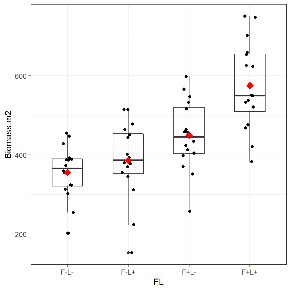
Figure 6.2: Boxplot and individual biomass values (black points) with treatment means (red diamonds)

Plotting the data and superimposing mean values produces the graph shown above. Now we are confident there is a difference in our sample means, we can begin a linear model to quantify this and test it against a null hypothesis.

If we use the FL column as a predictor then this is equivalent to a four-level one way ANOVA.

ls_1 <- lm(Biomass.m2 ~ FL, data = biomass)
summary(ls_1)

## 
## Call:
## lm(formula = Biomass.m2 ~ FL, data = biomass)
## 
## Residuals:
##      Min       1Q   Median       3Q      Max 
## -233.619  -42.842    1.356   67.961  175.381 
## 
## Coefficients:
##             Estimate Std. Error t value Pr(>|t|)    
## (Intercept)   355.79      23.14  15.376  < 2e-16 ***
## FLF-L+         30.12      32.72   0.921  0.36095    
## FLF+L-         93.69      32.72   2.863  0.00577 ** 
## FLF+L+        219.23      32.72   6.699 8.13e-09 ***
## ---
## Signif. codes:  0 '***' 0.001 '**' 0.01 '*' 0.05 '.' 0.1 ' ' 1
## 
## Residual standard error: 92.56 on 60 degrees of freedom
## Multiple R-squared:  0.4686, Adjusted R-squared:  0.442 
## F-statistic: 17.63 on 3 and 60 DF,  p-value: 2.528e-08

We can see that the control treatment (F- L-) is the intercept with a mean of 356g and standard error of 23g. The Light treatment adds an average of 30g to the biomass (but this close to the standard error of this estimated mean difference - 32.72g). In contrast the addition of fertiliser adds 93g to the biomass.

If we wanted to get the precise confidence intervals we could use broom::tidy(ls_1, conf.int = T) or confint(ls1).

We can visualise these differences with a coefficient plot, and see clearly that adding light by itself produce a slight increase in the mean biomass of our samples but the 95% confidence interval includes zero, so we don't have any real confidence that this is a consistent/true effect.

GGally::ggcoef_model(ls_1,
                      show_p_values=FALSE,
                      signif_stars = FALSE,
                     conf.level=0.95)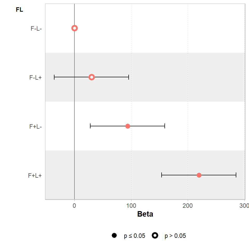

Figure 18.1: Effects of light and fertiliser treatments on biomass relative to an untreated control (error bars = 95% CI)

But what about the fourth level - combined fertiliser and light treatments? If there is no interaction (combined effect) between light and fertiliser then we would expect the average biomass difference caused by the light and the and the average biomass difference caused by fertiliser to add together to approximately the value found in the combined treatment.

In other words if one treatment has an effect size of A, and another treatment has an effect size of B, then ANOVA predicts that in combination the effect size of the combined treatments is A + B.

# combine the average mean differences of the light effect and fertiliser effect
coef(ls_1)[2] + coef(ls_1)[3] 

# compare this to the average difference of the combined treatment
coef(ls_1)[4]

##   FLF-L+ 
## 123.8187 
##  FLF+L+ 
## 219.225

In this example we can see clearly that combining the separate treatments does not add up to the combined value. The mean biomass of the combined treatment is well above the additive prediction.

The mean biomass of the combined treatment is well above what we would expect from the additive effects alone. This suggests there may be a positive interaction (that light and fertiliser treatments produce a sum effect that is greater than could be predicted by looking at their individual effects).

Using our one-way ANOVA design we are able to accurately estimate the mean difference between the controlled group and the combined treatment group. But we cannot really say anything concrete about the strength of the interaction effect e.g. is their a true interaction? how confident can we be in this effect? How does the strength of the interaction effect compare to the main effects?

In contrast to the one-way ANOVA approach, a factorial design lets us test and compare additive effects and interaction effects

18.4 Testing for interactions

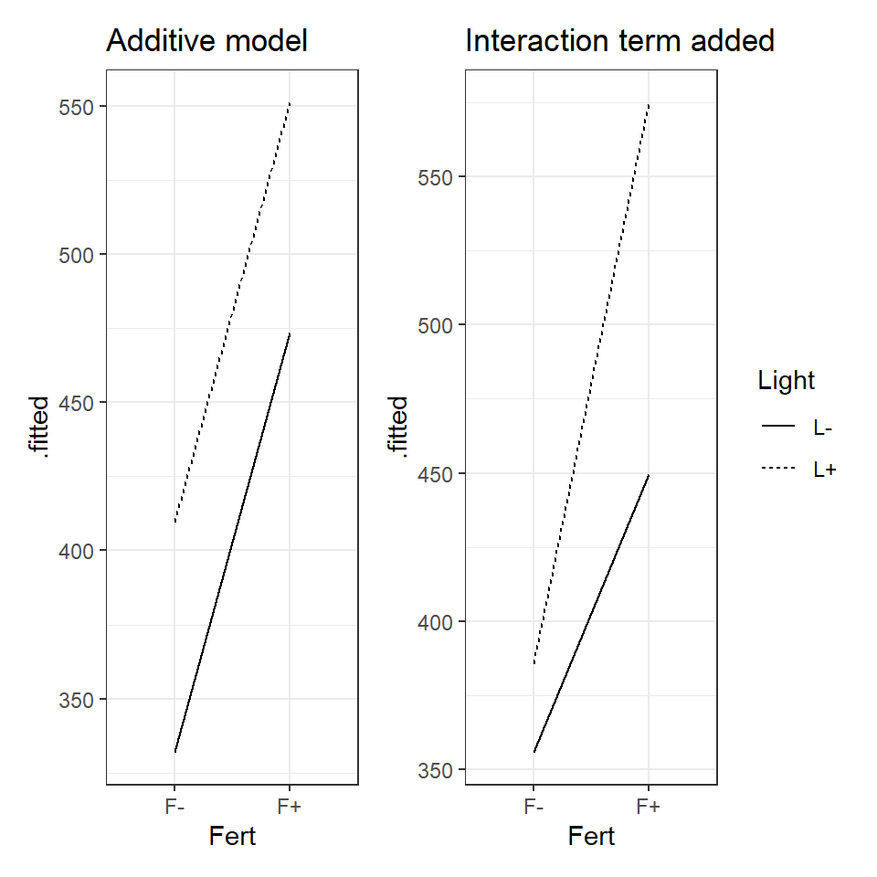
Figure 18.2: Left an illustration of an additive model, Right an illustration of a model with an interaction effect.

When the data can be best explained by an additive model, we expect new terms to shift the intercept up or down but the slope of the line to remain the same. An interaction effect changes the relationship as such we should see different gradients.

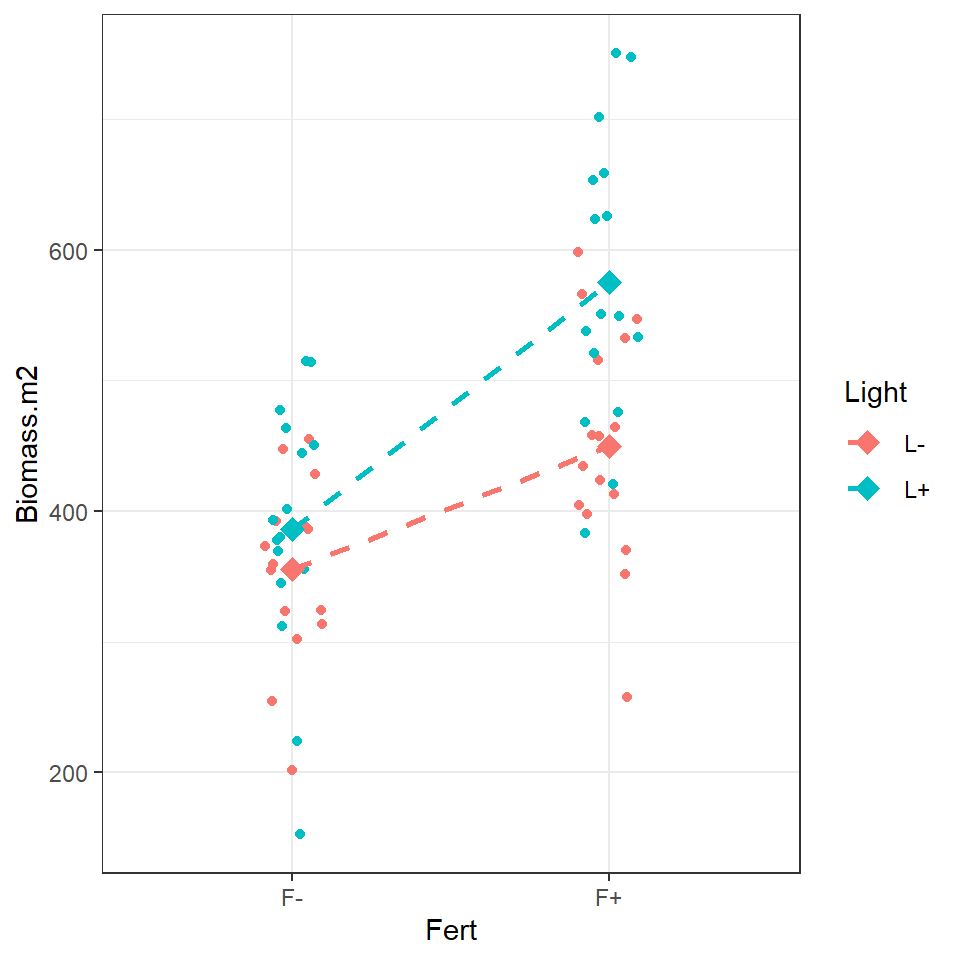
Look at the figure and determine whether you think there is evidence for an interaction effect?

biomass %>% ggplot(aes(x=Fert, y=Biomass.m2, colour = Light, fill = Light, group = Light))+
    geom_jitter(width=0.1) +
    stat_summary(
        geom = "point",
        fun = "mean",
        size = 3,
        shape = 23
    )+stat_summary(
        geom = "line",
        fun = "mean",
        size = 1, linetype = "dashed"
    )

To produce an interactive model, we need to use the separate factors for fertiliser and light rather than the single fl factor. When we make this model, we include the main effects of Light and Fert, if the additive model explains sufficient variance then this will be enough, but if we suspect an interaction term we add this as Light:Fert written out as follows:

ls_2 <- lm(Biomass.m2 ~ Fert + # main effect
             Light + # main effect
             Fert:Light, # interaction term
           data = biomass)

summary(ls_2)

## 
## Call:
## lm(formula = Biomass.m2 ~ Fert + Light + Fert:Light, data = biomass)
## 
## Residuals:
##      Min       1Q   Median       3Q      Max 
## -233.619  -42.842    1.356   67.961  175.381 
## 
## Coefficients:
##                Estimate Std. Error t value Pr(>|t|)    
## (Intercept)      355.79      23.14  15.376  < 2e-16 ***
## FertF+            93.69      32.72   2.863  0.00577 ** 
## LightL+           30.13      32.72   0.921  0.36095    
## FertF+:LightL+    95.41      46.28   2.062  0.04359 *  
## ---
## Signif. codes:  0 '***' 0.001 '**' 0.01 '*' 0.05 '.' 0.1 ' ' 1
## 
## Residual standard error: 92.56 on 60 degrees of freedom
## Multiple R-squared:  0.4686, Adjusted R-squared:  0.442 
## F-statistic: 17.63 on 3 and 60 DF,  p-value: 2.528e-08

Notice the estimates of the mean differences are the same as the previous one-way ANOVA model. The fourth line now indicates how much of an effect the two factors interacting changes the mean. Also note the standard error is larger, there is less power to accurately estimate an interaction over a main effect.

GGally::ggcoef_model(ls_2,
                      show_p_values=FALSE,
                      signif_stars = FALSE,
                     conf.level=0.95)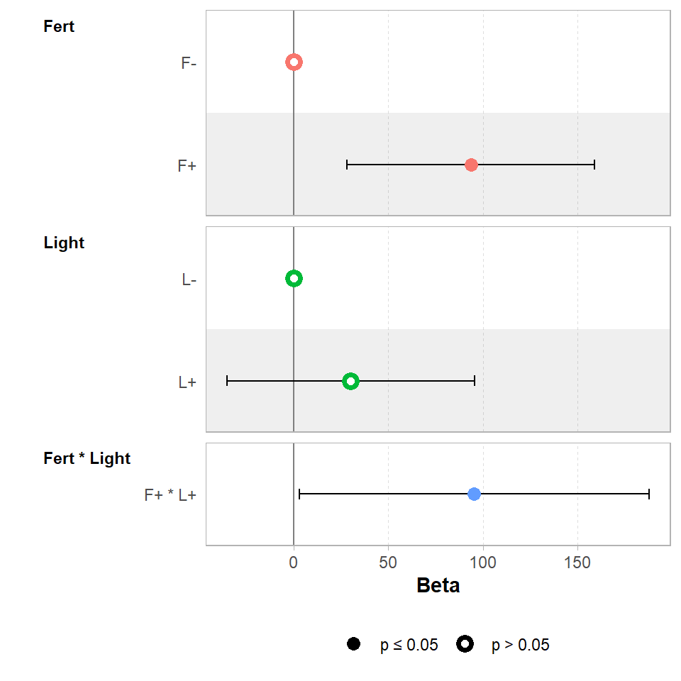

When we use a factorial combination, the last line of the table of coefficients estimates the size of the interaction effect at around 95g. So if combining the light and fertilisation treatments produced a biomass equivalent to their additive predictions, the estimate of the interaction would be zero. Instead it is 95g more than we would expect from the additive effects alone. This means in order to work out the estimated biomass for the treatment of light and fertiliser we must sum the additive effects of Light+ Fert and the interaction effect Light:Fert.

18.4.1 Model estimates and confidence intervals

When we compare this to our one-way ANOVA model, we must add the single terms and the interaction term, this should add up to the combined treatment from our first model:

# model 1
coef(ls_1)[4]

# model 2
coef(ls_2)[2] + coef(ls_2)[3] + coef(ls_2)[4]

##  FLF+L+ 
## 219.225 
##  FertF+ 
## 219.225

Don't make the mistake of looking at the main effect of light treatment, and reporting there is no effect because the uncertainty intervals cross zero. The main effect of light gives the average effect across the two fertiliser treatments. However, because of the interaction effect, we know this doesn't tell the whole story - whether light has an effect depends on whether fertiliser has been applied.

So, if you have a significant interaction term, you must consider the main effects, regardless of whether they are significant on their own.

18.5 ANOVA tables

So you have made a linear model with an interaction term, how do you report whether this interaction is significant? How do you report the main effect terms when there is an interaction present?

1. Start with the interaction

In previous chapters we ran the anova() function directly on our linear model. This works well for simple & 'balanced' designs (there are equal sample sizes in each level of a factor), but can be misleading with 'unbalanced' designs or models with complex interactions.

In order to report an F statistic for the interaction effect, we need to carry out an F-test of two models, one with and one without the interaction effect. This is easy with the function drop1()

drop1(ls_2, test = "F")

	Df	Sum of Sq	RSS	AIC	F value	Pr(>F)
<none>	NA	NA	513997.7	583.4298	NA	NA
Fert:Light	1	36409.41	550407.1	585.8099	4.250144	0.0435871

This F-test is testing the null hypothesis that there is no true interaction effect. The significance test rejects the null hypothesis (just). The drop1() function also provides the Akaike information criterion (AIC), an alternative method of model selection (more on this later).

We could now write this up as follows:

There was an interactive effect of light and fertiliser treatments (ANOVA F_1,60 = 4.25, P = 0.044) in which combining treatments produced substantially more biomass (95.4g [95% CI: 2.8 - 188]) than expected from the additive effects alone (Fertiliser 93.7g [28.2 - 159.2], Light 30.1g [-35.3 - 95.6]).

Do not make the mistake of just reporting the statistics, the interesting bit is the size of the effect (estimate) and the uncertainty (confidence intervals).

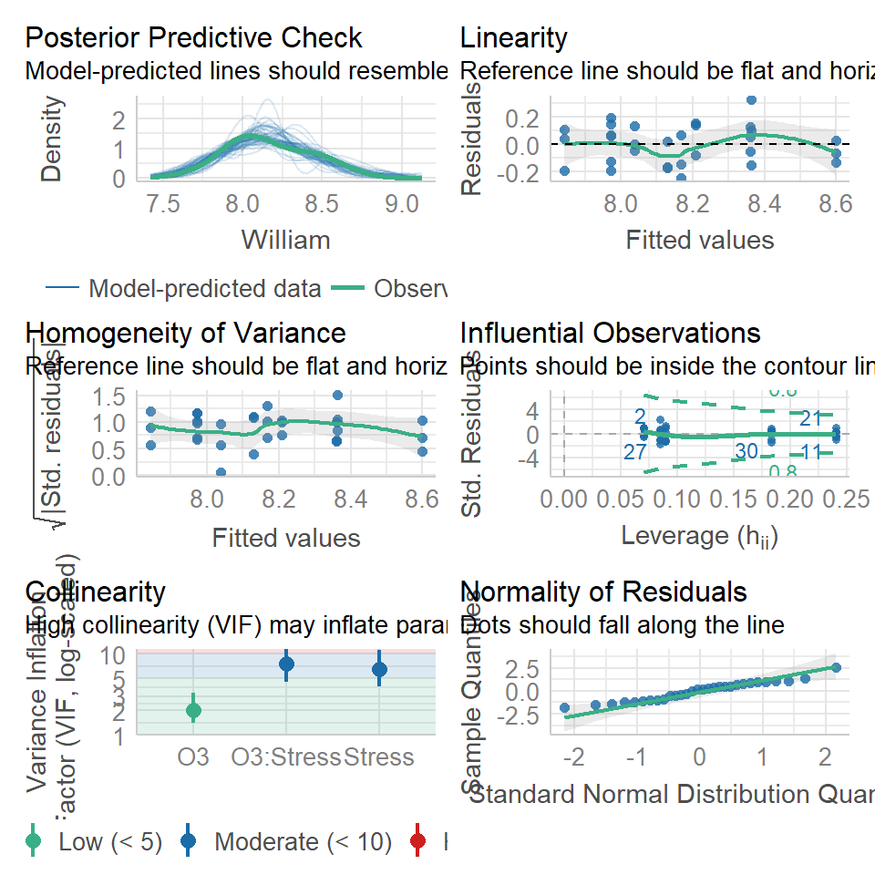
Remember to check the assumptions of your full model

2. Main effects

A good thing about the drop1() function is that if there are interactions in the model, it stops there. This is because if the interaction effect is significant, then the main effects must be included, even if they aren't significant on their own. We can make further models to test the main effects but these are less important because we already know the interaction term provides the main result.

If we decide to include reports of the main effect then estimates and confidence intervals should come from the full model, but we need to produce an interaction free model to produce accurate F-values (especially for unbalanced designs, see below).

# we have to remove the interaction term before we can keep using drop1()

ls_3 <- lm(Biomass.m2 ~ Fert + Light, data = biomass)

drop1(ls_3, test = "F")

	Df	Sum of Sq	RSS	AIC	F value	Pr(>F)
<none>	NA	NA	550407.1	585.8099	NA	NA
Fert	1	319889.22	870296.4	613.1332	35.45238	0.0000001
Light	1	96915.47	647322.6	594.1899	10.74086	0.0017322

You can use this reduced model to get F values, BUT reports of estimates should come from the full model.

18.6 Balanced/Unbalanced designs

In an unbalanced design when you run the anova() function on your model, the order in which your variables were included can have an effect e.g.

lm(Fert + Light) would give a different anova table to

lm(Light + Fert)

In the examples above, you are unlikely to find much of a difference between running the drop1() function or anova() on the complex or reduced models. This is because these designs are 'balanced' (equal numbers in each level of a predictor). When designs are not balanced then the order matters when we use anova() - this is because the sum of squares is calculated sequentially (in the order of the formula), and so we could get different results depending on the order in which we assemble predictors into our model!

18.6.1 Practice

Let's start by making a deliberately unbalanced dataset

# make three vectors and combine them into a new tibble

height <- c(50,57,91,94,102,110,57,71,85,105,120)
size <- c(rep("small", 2), rep("large", 4), rep("small", 3), rep("large", 2))
treatment <- c(rep("Control", 6), rep("Removal", 5))

unbalanced <- tibble(height, size, treatment)

unbalanced

height	size	treatment
50	small	Control
57	small	Control
91	large	Control
94	large	Control
102	large	Control
110	large	Control
57	small	Removal
71	small	Removal
85	small	Removal
105	large	Removal
120	large	Removal

18.7 Activity 1: Sums of Squares

Task

Produce a linear model testing size and treatment against height. Try making two models swapping the order for including the two predictors and compare them with anova()

Solution

model_1 <- lm(height ~ treatment + size, data = unbalanced)
anova(model_1)

model_2 <- lm(height ~ size + treatment, data = unbalanced)
anova(model_2)

	Df	Sum Sq	Mean Sq	F value	Pr(>F)
treatment	1	35.34545	35.34545	0.3724701	0.5585952
size	1	4846.04211	4846.04211	51.0675541	0.0000975
Residuals	8	759.15789	94.89474	NA	NA

	Df	Sum Sq	Mean Sq	F value	Pr(>F)
size	1	4291.2121	4291.21212	45.220760	0.0001489
treatment	1	590.1754	590.17544	6.219264	0.0372980
Residuals	8	759.1579	94.89474	NA	NA

Compare these two anova tables. Same data, same predictors, but a different conclusion just because of the order the terms were included in the model!

Task

Now compare your two models with the drop1() function

Solution

drop1(model_1)
drop1(model_2)

	Df	Sum of Sq	RSS	AIC
<none>	NA	NA	759.1579	52.57746
treatment	1	590.1754	1349.3333	56.90418
size	1	4846.0421	5605.2000	72.56910

	Df	Sum of Sq	RSS	AIC
<none>	NA	NA	759.1579	52.57746
size	1	4846.0421	5605.2000	72.56910
treatment	1	590.1754	1349.3333	56.90418

Because the drop1 function drops one term from the model, then adds it back in and drops a new one it doesn't matter what order they were included.

18.8 post-hoc

In this example it is unnecessary to spend time looking at pairwise comparisons between the four possible levels, the interesting finding is to report the strength of the interaction effect. But it is possible to generate estimated means, and produce pairwise comparisons with the emmeans() package

emmeans::emmeans(ls_2, specs = pairwise ~ Light + Fert + Light:Fert) %>% 
  confint()
# including the argument pairwise in front of the ~ prompts the post-hoc pairwise comparisons.
 # $emmeans contains the estimate mean values for each possible combination (with confidence intervals)
 # $ contrasts contains tukey test post hoc comparisons between levels

## $emmeans
##  Light Fert emmean   SE df lower.CL upper.CL
##  L-    F-      356 23.1 60      310      402
##  L+    F-      386 23.1 60      340      432
##  L-    F+      449 23.1 60      403      496
##  L+    F+      575 23.1 60      529      621
## 
## Confidence level used: 0.95 
## 
## $contrasts
##  contrast          estimate   SE df lower.CL upper.CL
##  (L- F-) - (L+ F-)    -30.1 32.7 60     -117    56.35
##  (L- F-) - (L- F+)    -93.7 32.7 60     -180    -7.22
##  (L- F-) - (L+ F+)   -219.2 32.7 60     -306  -132.75
##  (L+ F-) - (L- F+)    -63.6 32.7 60     -150    22.90
##  (L+ F-) - (L+ F+)   -189.1 32.7 60     -276  -102.63
##  (L- F+) - (L+ F+)   -125.5 32.7 60     -212   -39.06
## 
## Confidence level used: 0.95 
## Conf-level adjustment: tukey method for comparing a family of 4 estimates

18.9 Continuous Linear Models

The previous section looked at an interaction between two categorical variables, we can also examine interactions between a factor and a continuous variable. Often referred to as ANCOVA.

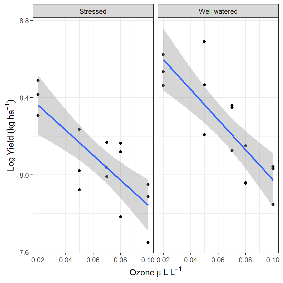
pollution <- read_csv(here::here("book", "files", "pollution.csv"))

The data is from an experimental study of the effects of low-level atmospheric pollutants and drought on agricultural yields. The experiment aimed to see how the yields soya bean (William variety), were affected by stress and Ozone levels. Your task is to first determine whether there is any evidence of an interaction effect, and if not drop this term from your model and then report the estimates and confidence intervals from the simplified model.

18.10 Activity 2: Build your own analysis

Try and make as much progress as you can without checking the solutions. Click on the boxes when you need help/to check your working

Task

Explore the data!

Solution

# check the structure of the data
glimpse(pollution)

# check data is in a tidy format
head(pollution)

# check variable names
colnames(pollution)

# check for duplication
pollution %>% 
  duplicated() %>% 
  sum()

# check for typos - by looking at impossible values
# quick summary

summary(biomass)

# check for typos by looking at distinct characters/values
pollution %>% 
  distinct(Stress)


# missing values
biomass %>% 
  is.na() %>% 
  sum()

## Rows: 30
## Columns: 4
## $ Stress  <chr> "Well-watered", "Well-watered", "Well-watered", "Well-watered"~
## $ SO2     <dbl> 0.00, 0.00, 0.00, 0.00, 0.00, 0.02, 0.02, 0.02, 0.02, 0.02, 0.~
## $ O3      <dbl> 0.02, 0.05, 0.07, 0.08, 0.10, 0.02, 0.05, 0.07, 0.08, 0.10, 0.~
## $ William <dbl> 8.623533, 8.690642, 8.360071, 8.151910, 8.032685, 8.535426, 8.~

Stress	SO2	O3	William
Well-watered	0.00	0.02	8.623533
Well-watered	0.00	0.05	8.690642
Well-watered	0.00	0.07	8.360071
Well-watered	0.00	0.08	8.151910
Well-watered	0.00	0.10	8.032685
Well-watered	0.02	0.02	8.535426

## [1] "Stress"  "SO2"     "O3"      "William"
## [1] 0
##      Fert              Light                FL              Biomass.m2   
##  Length:64          Length:64          Length:64          Min.   :152.3  
##  Class :character   Class :character   Class :character   1st Qu.:370.1  
##  Mode  :character   Mode  :character   Mode  :character   Median :425.9  
##                                                           Mean   :441.6  
##                                                           3rd Qu.:517.2  
##                                                           Max.   :750.4

Stress
Well-watered
Stressed

## [1] 0

Task

Visualise the data

Solution

pollution %>% 
  ggplot(aes(x = O3, y = William))+
  geom_point()+
  geom_smooth(method = "lm")+
  facet_wrap(~ Stress)+
    labs(x = expression(paste(Ozone~mu~L~L^-1)),
       y = expression(paste(Log~Yield~(kg~ha^-1))))

Task

Model the data

Solution

William_ls1 <- lm(William ~ O3 + Stress + O3:Stress, data = pollution)

William_ls1 %>% 
    broom::tidy(conf.int = T)

term	estimate	std.error	statistic	p.value	conf.low	conf.high
(Intercept)	8.4902296	0.0974956	87.0832015	0.0000000	8.2898245	8.6906347
O3	-6.4671581	1.4014008	-4.6147812	0.0000929	-9.3477788	-3.5865375
StressWell-watered	0.2642307	0.1378796	1.9163870	0.0663707	-0.0191849	0.5476463
O3:StressWell-watered	-1.3472822	1.9818801	-0.6798001	0.5026393	-5.4210950	2.7265306

It looks as though there is no strong evidence here for an interaction effect, but before we proceed any further we should check that the model is a good fit for our data.

18.10.1 Check the model fit

Task

Check the residuals of your model

Solution

performance::check_model(William_ls1)

18.10.2 Simplify the model

Task

Everything looks pretty good, so now we could go ahead and simplify our model.

Solution

Testing that dropping the interaction term does not significantly reduce the variance explained

drop1(William_ls1, test = "F")

	Df	Sum of Sq	RSS	AIC	F value	Pr(>F)
<none>	NA	NA	0.5698523	-110.9073	NA	NA
O3:Stress	1	0.0101286	0.5799809	-112.3787	0.4621281	0.5026393

18.10.2.1

Making a simpler model

William_ls2 <- lm(William ~ O3 + Stress, data = pollution) 

18.10.2.2

Get the F values of the simpler model

drop1(William_ls2, test = "F")

	Df	Sum of Sq	RSS	AIC	F value	Pr(>F)
<none>	NA	NA	0.5799809	-112.37872	NA	NA
O3	1	1.1381194	1.7181003	-81.79934	52.98317	0.0000001
Stress	1	0.2376424	0.8176233	-104.07653	11.06303	0.0025466

18.10.2.3

Report the estimates and confidence intervals of the new model

William_ls2 %>% 
    broom::tidy(conf.int = T)

term	estimate	std.error	statistic	p.value	conf.low	conf.high
(Intercept)	8.5333427	0.0733079	116.404189	0.0000000	8.3829273	8.6837580
O3	-7.1407992	0.9810200	-7.278954	0.0000001	-9.1536861	-5.1279124
StressWell-watered	0.1780046	0.0535173	3.326113	0.0025466	0.0681962	0.2878131

Task

Write up the results

Solution

I hypothesised that plants under stress might react more negatively to pollution than non-stressed plants, however when tested I found no evidence of a negative interation effect between stress and Ozone levels (F_1,27 = 0.4621, P = 0.5). Individually however, while well-watered plants had higher yields than stressed plants (mean 0.178 [95% CI: 0.0682 - 0.288]) (F_1,28 = 11, P = 0.003), there was a much larger effect of Ozone, where every unit increase (\(\mu\)L L^-1) produced a mean decrease in yield of 7.14 kg ha^-1 [5.13 - 9.15] (F_1,28 = 53, P < 0.001).

18.11 Summary

• Always have a good hypothesis for including an interaction

• When models have significant interaction effects you must always consider the main terms even if they are not significant by themselves

• Report F values from interactions as a priority

• IF interactions are significant then estimates should come from the full model, while F-values should come from a reduced model (for main effects). IF interaction terms are not significant they can be removed (model simplification).

• Use drop1() to avoid mistakes when using an unbalanced experiment design

• Always report estimates and effect sizes - this is the important bit - and easy to lose sight of when models get more complicated