7 Markdown
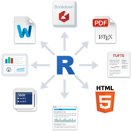
R Markdown is a widely-used tool for creating automated, reproducible, and share-worthy outputs, such as reports. It can generate static or interactive outputs, in Word, pdf, html, Powerpoint slides, and many other formats.
An R Markdown script combines R code and text such that the script actually becomes your output document. You can create an entire formatted document, including narrative text (can be dynamic to change based on your data), tables, figures, bullets/numbers, bibliographies, etc.
Documents produced with Rmarkdown, allow analyses to be included easily - and make the link between raw data, analysis & and a published report completely reproducible.
With Rmarkdown we can make reproducible html, word, pdf, powerpoints or websites and dashboards3
To make your Rmd publish - hit the knit button at the top of the doc
7.0.1 Format
Go to RStudio Cloud and open your workspace from last time.
Follow the instructions carefully - and assemble your Rmarkdown file bit by bit - when prompted to 'knit' the document do it. We will then observed the results and might make changes.
7.1 Background to Rmarkdown
Markdown is a “language” that allows you to write a document using plain text, that can be converted to html and other formats. It is not specific to R. Files written in Markdown have a ‘.md’ extension.
R Markdown: is a variation on markdown that is specific to R - it allows you to write a document using markdown to produce text and to embed R code and display their outputs. R Markdown files have ‘.Rmd’ extension.
rmarkdown - the package: This is used by R to render the .Rmd file into the desired output. It’s focus is converting the markdown (text) syntax, so we also need…
knitr: This R package Xie (2021a) will read the code chunks, execute it, and ‘knit’ it back into the document. This is how tables and graphs are included alongside the text.
Pandoc: Finally, pandoc actually convert the output into word/pdf/powerpoint etc. It is a software separate from R but is installed automatically with RStudio.
Most of this process happens in the background (you do not need to know all these steps!) and it involves feeding the .Rmd file to knitr, which executes the R code chunks and creates a new .md (Markdown) file which includes the R code and its rendered output.
The .md file is then processed by pandoc to create the finished product: a Microsoft Word document, HTML file, Powerpoint document, pdf, etc.
When using RStudio Cloud - all of these features are pre-loaded - if you take your R journey further in the future and install a copy of R and RStudio on your own computer you might have to do a little setting up to get this working (see Appendices).

7.2 Starting a new Rmd file
In RStudio, if you open a new R markdown file, start with ‘File’, then ‘New file’ then ‘R markdown…’.
R Studio will give you some output options to pick from. In the example below we select “HTML” because we want to create an html document. The title and the author names are not important. If the output document type you want is not one of these, don’t worry - you can just pick any one and change it in the script later.
7.3 Activity 1: Make an Rmarkdown file
Try your first "knit" to make a document.
Create a new Rmarkdown file. It comes prepopulated with some example text and code.
Save this (without changes) to the same location as your
.Rprojfile name itcontained_report_penguins.Rmd.We have moved from visualisation to reproducible report making.
Try your first knit just hit the button and watch it work - see how the R code chunks are processed.
Read the intro information below to learn more about how Markdown works.
The working directory for .rmd files is a little different to working with scripts.
With a .Rmd file, the working directory is wherever the Rmd file itself is saved.
For example if you have your .Rmd file in a subfolder ~/markdownfiles/markdown.Rmd the code for read_csv("data/data.csv") within the markdown will look for a .csv file in a subfolder called data inside the 'markdown' folder and not the root project folder where the .RProj file lives.
So we have two options when using .Rmd files
-
Don't put the .Rmd file in a subfolder and make sure it lives in the same directory as your .RProj file - that way relative filepaths are the same between R scripts and Rmarkdown files
-
Use the
herepackage to describe file locations - more later
7.4 R Markdown parts
An R Markdown document can be edited in RStudio just like a standard R script. When you start a new R Markdown script, RStudio tries to be helpful by showing a template which explains the different section of an R Markdown script.
The below is what appears when starting a new Rmd script intended to produce an html output.
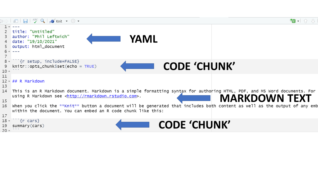
As you can see, there are three basic components to any Rmd file:
YAML
Markdown text
R code chunks.
7.4.1 YAML
Referred to as the ‘YAML metadata’ or just ‘YAML’, it is a recursive acronym that stands for "YAML ain't Markdown Language". It is found at the top of the R Markdown document. This section of the script will tell your Rmd file what type of output to produce, formatting preferences, and other metadata such as document title, author, and date.
In the example above, because we clicked that our default output would be an html file, we can see that the YAML says output: html_document. However we can also change this to say powerpoint_presentation or word_document or even pdf_document.
Can you edit the YAML in the Rmarkdown file in the markdown folder to have your name as author, today's date and the title of the file should be called "Penguins of the Palmer Archipelago, Antarctica".
7.4.2 Text
This is the narrative of your document, including the titles and headings. It is written in the “markdown” language, which is used across many different software.
Below are the core ways to write this text. See more extensive documentation available on R Markdown “cheatsheets” at the RStudio website4.
7.4.2.1 New lines
Uniquely in R Markdown, to initiate a new line, enter *two spaces** at the end of the previous line and then Enter/Return.
7.4.2.2 Text emphasis
Surround your normal text with these characters to change how it appears in the output.
Underscores (_text_) or single asterisk (*text*) to italicise
Double asterisks (**text**) for bold text
Back-ticks (` text `) to display text as code
The actual appearance of the font can be set by using specific templates (specified in the YAML metadata).
7.4.2.3 Titles and headings
A hash symbol in a text portion of a R Markdown script creates a heading. This is different than in a chunk of R code in the script, in which a hash symbol is a mechanism to comment/annotate/de-activate, as in a normal R script.
Different heading levels are established with different numbers of hash symbols at the start of a new line. One hash symbol is a title or primary heading. Two hash symbols are a second-level heading. Third- and fourth-level headings can be made with successively more hash symbols.
# First-level heading / Title

## Second level heading

### Third-level heading
7.4.2.4 Bullets and numbering
Use asterisks (*) to created a bullets list. Finish the previous sentence, enter two spaces, Enter/Return twice, and then start your bullets. Include a space between the asterisk and your bullet text. After each bullet enter two spaces and then Enter/Return. Sub-bullets work the same way but are indented. Numbers work the same way but instead of an asterisk, write 1), 2), etc. Below is how your R Markdown script text might look.
Here are my bullets (there are two spaces after this colon):
* Bullet 1 (followed by two spaces and Enter/Return)
* Bullet 2 (followed by two spaces and Enter/Return)
  * Sub-bullet 1 (followed by two spaces and Enter/Return)
  * Sub-bullet 2 (followed by two spaces and Enter/Return)
7.4.3 Code Chunks
Sections of the script that are dedicated to running R code are called “chunks”. This is where you may load packages, import data, and perform the actual data management and visualisation. There may be many code chunks, so they can help you organize your R code into parts, perhaps interspersed with text. To note: These ‘chunks’ will appear to have a slightly different background colour from the narrative part of the document.
Each chunk is opened with a line that starts with three back-ticks, and curly brackets that contain parameters for the chunk { }. The chunk ends with three more back-ticks.
```{r}
code goes here
```
You can create a new chunk by typing it out yourself, by using the keyboard shortcut “Ctrl + Alt + i” (or Cmd + Shift + r in Mac), or by clicking the green ‘insert a new code chunk’ icon at the top of your script editor.
Some notes about the contents of the curly brackets { }:
They start with ‘r’ to indicate that the language name within this chunk is R. It is possible to include other programming language chunks here such as SQL, Python or Bash.
After the r you can optionally write a chunk “name” – these are not necessary but can help you organise your work. Note that if you name your chunks, you should ALWAYS use unique names or else R will complain when you try to render.
After the language name and optional chunk name put a comma, then you can include other options too, written as tag=value, such as:
-
eval = FALSE to not run the R code
-
echo = FALSE to not print the chunk’s R source code in the output document
-
warning = FALSE to not print warnings produced by the R code
-
message = FALSE to not print any messages produced by the R code
-
include = either TRUE/FALSE whether to include chunk outputs (e.g. plots) in the document
-
out.width = and out.height = - size of ouput e.g. out.width = "75%"
-
fig.align = "center" adjust how a figure is aligned across the page
-
fig.show='hold' if your chunk prints multiple figures and you want them printed next to each other (pair with out.width = c("33%", "67%").
- A chunk header must be written in one line
```{r optional-name , eval = TRUE, echo = FALSE}

```- Try to avoid periods, underscores, and spaces. Use hyphens ( - ) instead if you need a separator.
Read more extensively about the knitr options here5.
There are also two arrows at the top right of each chunk, which are useful to run code within a chunk, or all code in prior chunks. Hover over them to see what they do.
7.5 Activity 2: Setting code chunks
Question 1. The global option for this document is set to show the R code used to render chunks
knitr::opts_chunk$set(echo = TRUE)
Question 2. Options set in individual code chunks override the global options
In the second chunk we see echo = FALSE and this has prevented the code from being printed, we only see the rendered output
Question 3. If we wanted to see the R code, but not its output we need to select what combo of code chunk options?
7.5.1 Global options
For global options to be applied to all chunks in the script, you can set this up within your very first R code chunk in the script.
This is very handy if you know you will want the majority of your code chunks to behave in the same way.
For instance, so that only the outputs are shown for each code chunk and not the code itself, you can include this command in the R code chunk (and set this chunk to include = false):
knitr::opts_chunk$set(echo = FALSE) Global options are useful, but each code block can still be individually set.
7.5.2 In-text code
You can also include minimal R code within back-ticks. Within the back-ticks, begin the code with “r” and a space, so RStudio knows to evaluate the code as R code. See the example below.
This book was printed on `r Sys.Date()`
When typed in-line within a section of what would otherwise be Markdown text, it knows to produce an r output instead:
This book was printed on 2023-10-10
7.6 Activity 3: Make some markdown edits
Having added some in-line code, try re-knitting your .Rmd file.
7.7 Activity 4: Generating a self-contained report from data
For a relatively simple report, you may elect to organize your R Markdown script such that it is “self-contained” and does not involve any external scripts.
Set up your Rmd file to 'read' the penguins data file.
Everything you need to run the R markdown is imported or created within the Rmd file, including all the code chunks and package loading. This “self-contained” approach is appropriate when you do not need to do much data processing (e.g. it brings in a clean or semi-clean data file) and the rendering of the R Markdown will not take too long.
In this scenario, one logical organization of the R Markdown script might be:
Set global knitr options
Load packages
Import data
Process data
Produce outputs (tables, plots, etc.)
Save outputs, if applicable (.csv, .png, etc.)
```{r, include=FALSE}
# GLOBAL KNITR OPTIONS ----
knitr::opts_chunk$set(echo = TRUE)
# ____________________----

# PACKAGES ----
library(tidyverse)

```
```{r}
# READ DATA ----
penguins <- read_csv("data/penguins_raw.csv")
head(penguins)
```
7.7.1 Heuristic file paths with here()
The package here Müller (2020) and its function here() (here::here()), make it easy to tell R where to find and to save your files - in essence, it builds file paths. It becomes especially useful for dealing with the alternate filepaths generated by .Rmd files, but can be used for exporting/importing any scripts, functions or data.
This is how here() works within an R project:
When the
herepackage is first loaded within the R project, it places a small file called “.here” in the root folder of your R project as a “benchmark” or “anchor”In your scripts, to reference a file in the R project’s sub-folders, you use the function
here()to build the file path in relation to that anchorTo build the file path, write the names of folders beyond the root, within quotes, separated by commas, finally ending with the file name and file extension as shown below
here()file paths can be used for both importing and exporting
So when you use here() wrapped inside other functions for importing/exporting (like read_csv() or ggsave()) if you include here() you can still use the RProject location as the root directory when 'knitting' Rmarkdown files, even if your markdown is tidied away into a separate sub-folder.
This means your previous relative filepaths should be replaced with:
```{r, include=FALSE}
# GLOBAL KNITR OPTIONS ----
knitr::opts_chunk$set(echo = TRUE)
# ____________________----

# PACKAGES ----
library(tidyverse)
library(here)

```
```{r, include=FALSE}
# READ DATA ----
penguins <- read_csv(here("data", "penguins_raw.csv"))
head(penguins)
```Try replacing your previous code with the examples above then re-knitting your .Rmd file.
You might want start using the here() from now on to read in and export data from scripts. Make sure you are consistent in whether you use here() heuristic file paths or relative file paths across all .R and .Rmd files in a project - otherwise you might encounter errors.
7.8 Activity 4: Can you change the global options of your Rmd file so that it doesn't display any code, warnings or messages?
Once you have made your edits to the chunk options try hitting 'knit' again.
7.9 ggplot
7.9.1 Size options for figures
Options fig.width and fig.height enable to set width and height of R produced figures. The default value is set to 7 (inches). When I play with these options, I prefer using only one of them (fig.width) in association with another one, fig.asp, which sets the height-to-width ratio of the figure. It’s easier in my mind to play with this ratio than to give a width and a height separately. The default value of fig.asp is NULL but I often set it to (0.8), which often corresponds to the expected result.
Size options of figures produced by R have consequences on relative sizes of elements in this figures. For a ggplot2 figure, these elements will remain to the size defined in the used theme, whatever the chosen size of the figure. Therefore a huge size can lead to a very small text and vice versa.
The base font size is 11 pts by default. You can change it with the base_size argument in the theme you’re using.
The code below is likely to produce an error and cause the document to fail to knit. From the error message can you work out what is missing from our code that is causing this? Hint - there is a difference in the column names we are asking for and the ones in the actual spreadsheet we just imported
# snake_case names need to be made

penguins <- janitor::clean_names(penguins)
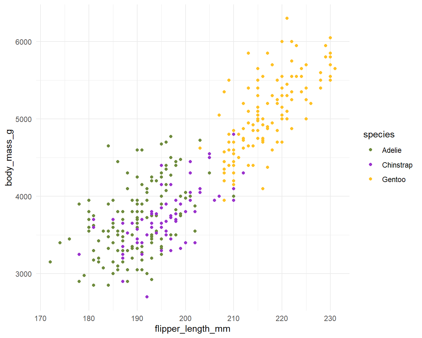
penguin_colours <- c("darkolivegreen4", "darkorchid3", "goldenrod1")

plot <- penguins %>%
  ggplot(aes(x=flipper_length_mm,
             y = body_mass_g))+
  geom_point(aes(colour=species))+
  scale_color_manual(values=penguin_colours)+
  theme_minimal(base_size = 11)
```{r fig.asp = 0.8, fig.width = 3}
plot
# figure elements are too big
```
```{r fig.asp = 0.8, fig.width = 10}
plot
# figure elements are too small
```
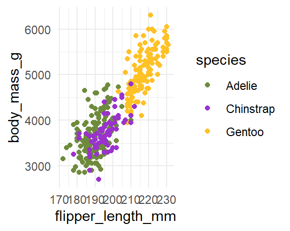
To find the result you like, you’ll need to combine sizes set in your theme and set in the chunk options. With my customised theme, the default size (7) looks good to me.
```{r fig.asp = 0.8, fig.width = 7}
plot
```
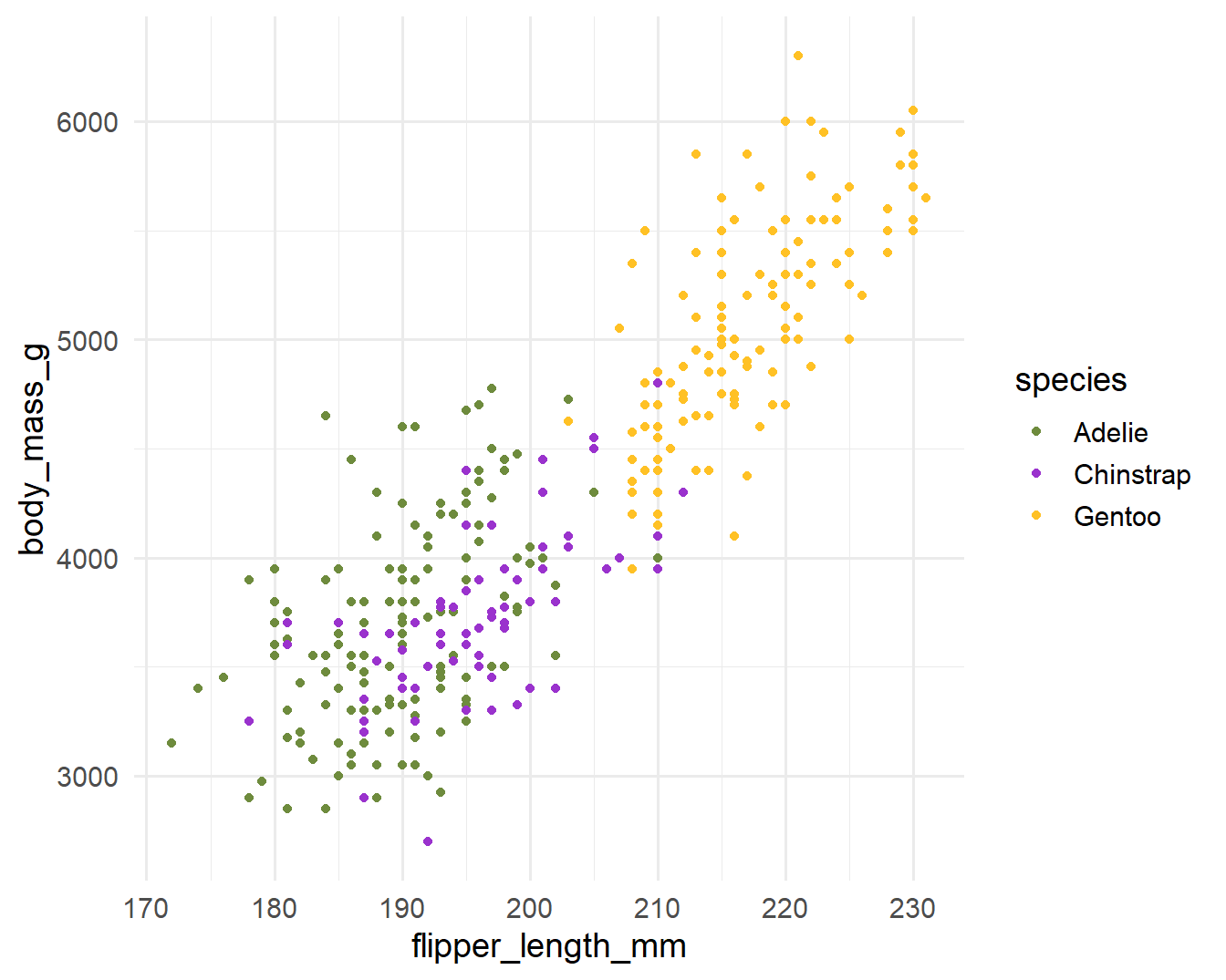
When texts axis are longer or when figures is overloaded, you can choose bigger size (8 or 9) to relatively reduce the figure elements. it’s worth noting that for the text sizes, you can also modify the base size in your theme to obtain similar figures.
```{r fig.asp = 0.8, fig.width = 7}
plot + theme(base_size = 14)
# figure width stays the same, but modify the text size in ggplot
```
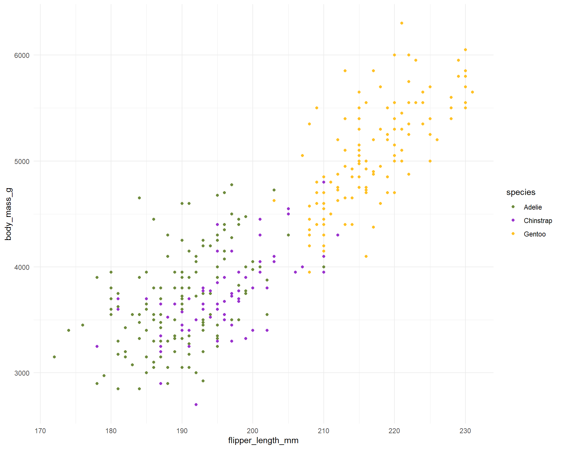
7.9.2 Size of final figure in document
Figures made with R in a R Markdown document are exported (by default in png format) and then inserted into the final rendered document. Options out.width and out.height enable us to choose the size of the figure in the final document.
It is rare I need to re-scale height-to-width ratio after the figures were produced with R and this ratio is kept if you modify only one option therefore I only use out.width. i like to use percentage to define the size of output figures. For example with a size set to 50%
```{r fig.asp = 0.8, fig.width = 7, out.width = "50%"}
plot
# The final rendered size of the image changes according to out.width
```
7.9.3 Changing default values of chunk options
You can also change default values of chunk options by writing this at the beginning of your R Markdown document.
```{r setup, include=FALSE}
knitr::opts_chunk$set(
 fig.width = 6,
 fig.asp = 0.8,
 out.width = "80%"
)
```
These values will be applied for all chunks unless you specify other value in a chunk locally. You can set values often used (which differ from the default one) and avoid repeating them for each chunk.
7.10 Static images
You can include images in your R Markdown in several ways:
knitr::include_graphics("path/to/image.png")
# choose ONE of these
knitr::include_graphics("../images/darwin.png")

knitr::include_graphics(here("images", "darwin.png")
7.11 Tables
7.11.1 Markdown tables
| Syntax      | Description |
| ----------- | ----------- |
| Header      | Title       |
| Paragraph   | Text        |
Which will render as this
| Syntax | Description |
|---|---|
| Header | Title |
| Paragraph | Text |
7.11.2 knitr::kable()
To create and manage able objects, we first pass the data frame through the kable() function from the knitr package. The package kableExtra Zhu (2020) gives us lots of extra styling options.6
Can you get this working? Add the library call for kableExtra to the first chunk of your Rmd file, then make a chunk for the below at the bottom of your file and hit knit to test.
penguins %>%
  group_by(species) %>%
  summarise(`Body Mass (g)`= mean(body_mass_g, na.rm = T),
            `Flipper Length (mm)`= mean(flipper_length_mm, na.rm = T)) %>%
  kbl(caption = "Mean Body mass (g) and flipper length (mm) for three species of Penguin in the Palmer Archipelago") %>%
kable_styling(bootstrap_options = "striped", full_width = F, position = "left")| species | Body Mass (g) | Flipper Length (mm) |
|---|---|---|
| Adelie | 3700.662 | 189.9536 |
| Chinstrap | 3733.088 | 195.8235 |
| Gentoo | 5076.016 | 217.1870 |
7.11.3 gt()
The gt Iannone et al. (2021) package is all about making it simple to produce nice-looking display tables in HTML (so won't work for LaTex). It has a lot of customisation options.
penguins %>%
    group_by(species) %>%
    summarise(`Body Mass (g)`= mean(body_mass_g, na.rm = T),
`Flipper Length (mm)`= mean(flipper_length_mm, na.rm = T)) %>% gt::gt()| species | Body Mass (g) | Flipper Length (mm) |
|---|---|---|
| Adelie | 3700.662 | 189.9536 |
| Chinstrap | 3733.088 | 195.8235 |
| Gentoo | 5076.016 | 217.1870 |
You won't be able to see these tables unless you try re-knitting your .Rmd file.
7.12 Source files
One variation of the “self-contained” approach is to have R Markdown code chunks “source” (run) other R scripts.
This can make your R Markdown script less cluttered, more simple, and easier to organize. It can also help if you want to display final figures at the beginning of the report.
In this approach, the final R Markdown script simply combines pre-processed outputs into a document. We already used the source() function to feed R objects from one script to another, now we can do the same thing to our report.
The advantage is all the data cleaning and organising happens "elsewhere" and we don't need to repeat our code. If you make any changes in your analysis scripts, these will be reflected by changes in your report the next time you compile (knit) it.
source("scripts/your-script.R")
Don't try using here() unless ALL of your script dependencies ALSO use this. When knitting an Rmd file it treats the absolute file path as relative to the .Rmd file (even when running scripts written outside of the document).
This is why it's usually simpler to save your .Rmd file in the same place as your .RProj file
7.13 Activity 5: Connecting scripts and reports
Create a new Rmarkdown file.
Save this (without changes) to the same folder as your
.Rprojfile and call it03_linked_report_penguins.Rmd.
We will now source the pre-written scripts for data loading and wrangling in your R project, just use the source command to read in this script - then you can call objects made externally - in this case a penguin plot - put the code block in and hit knit.
```{r setup, include=FALSE}
# GLOBAL KNITR OPTIONS ----
knitr::opts_chunk$set(echo = TRUE)
# ____________________----

# PACKAGES ----
library(tidyverse)


```
```{r read-data, include=FALSE}
# READ DATA ----
source("scripts/02_visualisation_penguins.R")
```
```{r figure, include=FALSE}
(p1+p2)/p3+
plot_layout(guides = "collect")
```7.14 Activity 6: Test yourself
Let's make another reproducible report.
Make a new Rmarkdown or RNotebook file
YYYYMMDD_surname_5023Y_rmd_workshop.RmdMake any summary figure you want from the penguins data with
ggplotMake a summary table with
summariseand make it beautiful withkableExtraorgt()Write a few sentences explaining what you are presenting
Knit the report to html
Use chunk options to optimise your figure layout and text and make it so that raw code and rendered outputs are visible. An example of literate programming
7.14.1 Hygiene tips
I recommend having three chunks at the top of any document
Global chunk options
All packages
Reading data
```{r setup , include=FALSE}
knitr::opts_chunk$set(echo = TRUE,
                      fig.align = "center",
                      fig.width = 6,
                      fig.asp = 0.8,
                      out.width = "80%
                      )

```

```{r library}
library(tidyverse)
```

```{r read-data}
source("scripts/02_visualisation_penguins.R")
```
7.15 Common knit issues
Any of these issues will cause the Rmd document to fail to knit in its entirety. A failed knit is usually an easy fix, but needs you to READ the error message, and do a little detective work.
7.15.2 Not the right order
plot(my_table)

my_table <- table(mtcars$cyl)7.16 Visual editor
RStudio comes with a pretty nifty Visual Markdown Editor which includes:
Spellcheck
Easy table & equation insertion
Easy citations and reference list building
You can switch between modes with a button push, try it out!
7.17 Activity 7: Test yourself
Submit your final knitted report YYYYMMDD_surname_5023Y_rmd_workshop.html to Blackboard
You may need to send this to a zipped folder for submission at the Blackboard portal
Find the doi for the palmerpenguins Horst et al. (2020) package, and use the visual editor to easily include a reference in your report.
When completed and the document is reknit. Check the output document and your original markdown file + project space.
You should find a new file in your project space .bib and new conditions in your YAML?
7.18 Summing up Rmarkdown
7.18.1 What we learned
You have learned
How to use markdown with
knitrHow to embed R chunks, to produce code, figures and analyses
How to organise projects with
hereHow to knit to pdf and html outputs
How to make simple tables
How to size figure outputs for your documents
7.18.2 Further Reading, Guides and tips
The fully comprehensive guide