20 Generalized Linear Models
20.1 Motivation
In the previous workshop we have seen that linear models are a powerful modelling tool. However, we have to satisfy the following assumptions:
- A linear relationship between predictors and the mean response value.
- Variances are equal across all predicted values of the response (homoscedatic)
- Errors are normally distributed.
- Samples collected at random.
- No omitted variables of importance
If assumptions 1-3 are violated we can often transform our response variable to try and fix this (Box-Cox & transformation). However, in a lot of other cases this is either not possible (e.g binary output) or we want to explicitly model the underlying distribution (e.g count data). Instead, we can use Generalized Linear Models (GLMs) that let us change the error structure (assumption 3) to something other than a normal distribution.
20.2 Generalised Linear Models (GLMs)
Generalised Linear Models (GLMs) have:
A linear predictor.
An error/variance structure.
A link function (like an 'internal' transformation).
The first (1) should be familiar, its everything that comes after the ~ in a linear model formula. Or as an equation \(\beta_0 + \beta_1\). The second (2) should also be familiar, variance measures the error structure of the model \(\epsilon\). An ordinary least squares model uses the normal distribution, but GLMs are able to use a wider range of distributions including poisson, binomial and Gamma. The third component (3) is less familiar, the link function is the equivalent of a transformation in an ordinary least squares model. However, rather than transforming the data, we transform the predictions made by the linear predictors. Common link functions are log and square root.
Maximum Likelihood - Generalised Linear Models fit a regression line by finding the parameter values that best fit the model to the data. This is very similar to the way that ordinary least squares finds the line of best fit by reducing the sum of squared errors. In fact for data with normally distributed residuals, the particular form of maximum likelihood is least squares.
However the normal (gaussian) distribution will not be a good model for lots of other types of data, binary data, is a good example and one we will investigate in this workshop.
Maximum likelihood provides a more generalized approach to model fitting that includes, but is broader than, least squares.
An advantage of the least squares method we have been using is that we can generate precise equations for the fit of the line. In contrast the calculations for GLMs (which are beyond the scope of this course) are approximate, essentially multiple potential best fit lines are made and compared against each other.
You will see two main differences in a GLM output:
If the model is one where the mean and variance are calculated separately (e.g. for most normal distributions), uncertainty estimates use the t distribution; and when we compare complex to simplified models (using anova() or drop1()) we use the F-test.
However, when we provide distributions where the mean and variance are expected to change together (Poisson and Binomial), then we calculate uncertainty estimates using the z distribution, and compare models with the chi-square distribution.
The simple linear regression model we have used so far is a special cases of a GLM:
lm(height ~ weight)is equivalent to
glm(height ~ weight, family=gaussian(link=identity))Compared to lm(), the glm() function takes an additional argument called family, which
specifies the error structure and link function.
The default link function for the normal (Gaussian) distribution is the identity, where no transformation is neededi.e. for mean \(\mu\) we have:
\[ \mu = \beta_0 + \beta_1 X \]
Defaults are usually good choices (shown in bold below):
| Family | Link |
|---|---|
gaussian |
identity |
binomial |
logit, probit or cloglog
|
poisson |
log, identity or sqrt
|
Gamma |
inverse, identity or log
|
inverse.gaussian |
1/mu^2 |
quasibinomial |
logit |
quasipoisson |
log |
20.3 Workflow for fitting a GLM
- Exploratory data analysis
- Choose suitable error term
- Choose suitable mean function (and link function)
- Fit model
- Residual checks and model fit diagnostics
- Revise model (transformations etc.)
- Model simplification if required
- Check final model again
When you transform your data e.g. with a log or sqrt, this changes the mean and variance at the same time (everything gets squished down). This might be fine, but can lead to difficult model fits if you need to reduce unequal variance but this leads to a change (often curvature) in the way the predictors fit to the response variable.
GLMs model the mean and variability independently. So a link function produces a transformation between predictors and the mean, and the relationship between the mean and data points is modeled separately.
20.4 Poisson regression (for count data or rate data)
Count or rate data are ubiquitous in the life sciences (e.g number of parasites per microlitre of blood, number of species counted in a particular area). These type of data are discrete and non-negative. In such cases assuming our response variable to be normally distributed is not typically sensible. The Poisson distribution lets us model count data explicitly.
Recall the simple linear regression case (i.e a GLM with a Gaussian error structure and identity link). For the sake of clarity let's consider a single explanatory variable where \(\mu\) is the mean for Y:
\[ \begin{aligned} \mu & = \beta_0 + \beta_1X \end{aligned} \]
The mean function is unconstrained, i.e the value of \(\beta_0 + \beta_1X\) can range from \(-\infty\) to \(+\infty\). If we want to model count data we therefore want to constrain this mean to be positive only. Mathematically we can do this by taking the logarithm of the mean (the log is the default link for the Poisson distribution). We then assume our count data variance to be Poisson distributed (a discrete, non-negative distribution), to obtain our Poisson regression model (to be consistent with the statistics literature we will rename \(\mu\) to \(\lambda\)):
\[ \begin{aligned} Y & \sim \mathcal{Pois}(\lambda) \\ \log{\lambda} & = \beta_0 + \beta_1X \end{aligned} \]
Note - the relationship between the mean and the data is modelled by Poisson variance. The relationship between the predictors and the mean is modelled by a log transformation.
The Poisson distribution has the following characteristics:
- Discrete variable, defined on the range \(0, 1, \dots, \infty\).
- A single rate parameter \(\lambda\), where \(\lambda > 0\).
-
Mean = \(\lambda\)
- Variance = \(\lambda\)
So we model the variance as equal to the mean - as the mean increases so does the variance.
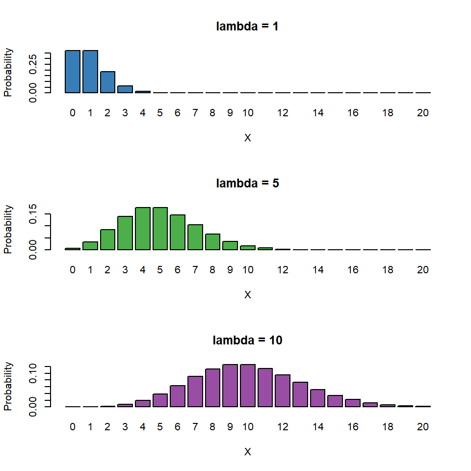

So for the Poisson regression case we assume that the mean and variance are the same. Hence, as the mean increases, the variance increases also (heteroscedascity). This may or may not be a sensible assumption so watch out! Just because a Poisson distribution usually fits well for count data, doesn't mean that a Gaussian distribution can't always work.
Recall the link function between the predictors and the mean and the rules of logarithms (if \(\log{\lambda} = k\)(value of predictors), then \(\lambda = e^k\)):
\[ \begin{aligned} \log{\lambda} & = \beta_0 + \beta_1X \\ \lambda & = e^{\beta_0 + \beta_1X } \end{aligned} \] Thus we are effectively modelling the observed counts (on the original scale) using an exponential mean function.
20.5 Example: Cuckoos

In a study by Kilner et al. (1999), the authors studied the begging rate of nestlings in relation to total mass of the brood of reed warbler chicks and cuckoo chicks. The question of interest is:
How does nestling mass affect begging rates between the different species?
cuckoo <- read_csv(here::here("book", "files", "cuckoo.csv"))
head(cuckoo)| Mass | Beg | Species |
|---|---|---|
| 9.637522 | 0 | Cuckoo |
| 10.229151 | 0 | Cuckoo |
| 13.103706 | 0 | Cuckoo |
| 15.217391 | 0 | Cuckoo |
| 16.231884 | 0 | Cuckoo |
| 20.120773 | 0 | Cuckoo |
The data columns are:
- Mass: nestling mass of chick in grams
- Beg: begging calls per 6 secs
- Species: Warbler or Cuckoo
ggplot(cuckoo, aes(x=Mass, y=Beg, colour=Species)) + geom_point()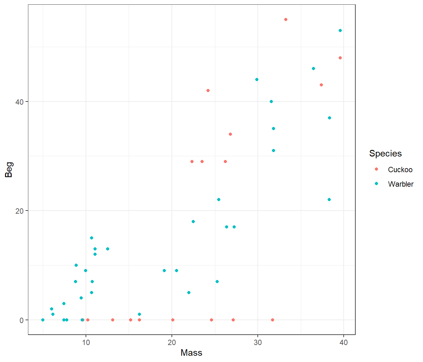
There seem to be a relationship between mass and begging calls and it could be different between species. It is tempting to fit a linear model to this data. In fact, this is what the authors of the original paper did; reed warbler chicks (solid circles, dashed fitted line) and cuckoo chick (open circles, solid fitted line):
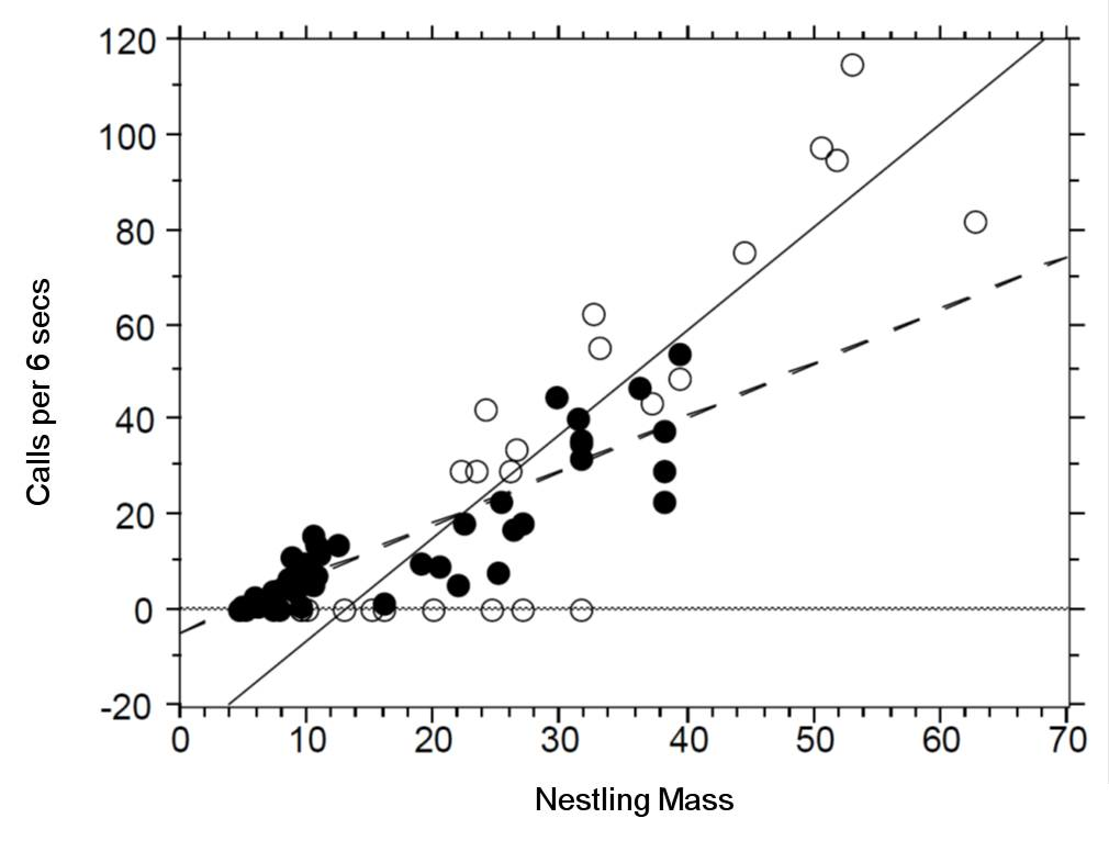
This model is inadequate. It is predicting negative begging calls within the range of the observed data, which clearly does not make any sense.
Let us display the model diagnostics plots for this linear model.
## Fit model
## There is an interaction term here, it is reasonable to think that how calling rates change with size might be different between the two species.
cuckoo_ls1 <- lm(Beg ~ Mass+Species+Mass:Species, data=cuckoo)
performance::check_model(cuckoo_ls1,
                         check = c("homogeneity",
                                   "qq"))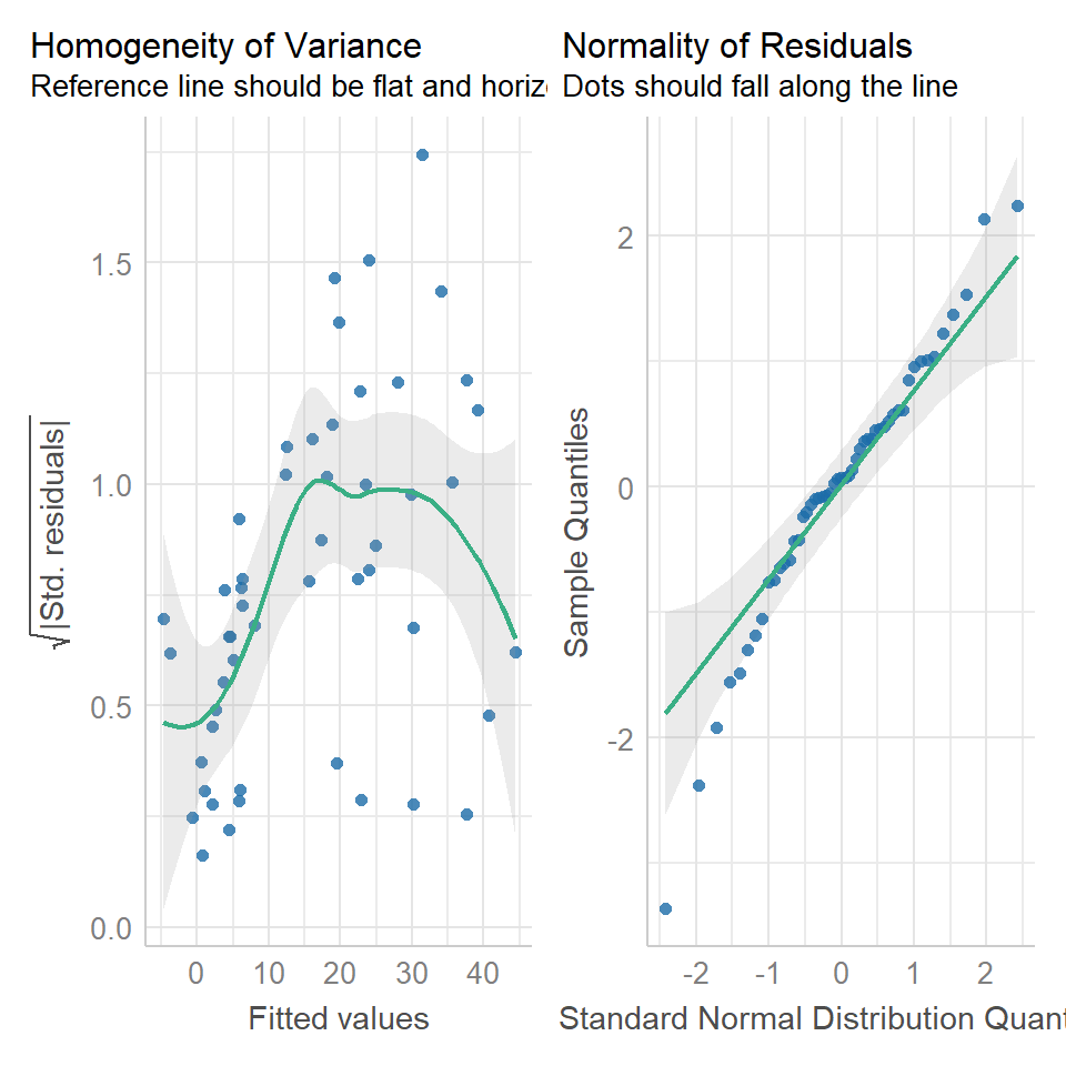
The residuals plot depicts a strong "funnelling" effect, highlighting that the model assumptions are violated. We should therefore try a different model structure.
The response variable in this case is a classic count data: discrete and bounded below by zero (i.e we cannot have negative counts). We will therefore try a Poisson model using the canonical log link function for the mean:
\[ \log{\lambda} = \beta_0 + \beta_1 M_i + \beta_2 S_i + \beta_3 M_i S_i \]
where \(M_i\) is nestling mass and \(S_i\) a dummy variable
\[ S_i = \left\{\begin{array}{ll} 1 & \mbox{if $i$ is warbler},\\ 0 & \mbox{otherwise}. \end{array} \right. \]
The term \(M_iS_i\) is an interaction term. Think of this as an additional explanatory variable in our model. Effectively it lets us have different slopes for different species (without an interaction term we assume that both species have the same slope for the relationship between begging rate and mass, and only the intercept differ).
The mean regression lines for the two species look like this:
- Cuckoo (\(S_i=0\))
\[ \begin{aligned} \log{\lambda} & = \beta_0 + \beta_1 M_i + (\beta_2 \times 0) + (\beta_3 \times M_i \times 0)\\ \log{\lambda} & = \beta_0 + \beta_1 M_i \end{aligned} \]
Intercept = \(\beta_0\), Gradient = \(\beta_1\)
Warbler (\(S_i=1\))
\[ \begin{aligned} \log{\lambda} & = \beta_0 + \beta_1 M_i + (\beta_2 \times 1) + (\beta_3 \times M_i \times 1)\\ \log{\lambda} & = \beta_0 + \beta_1 M_i + \beta_2 + \beta_3M_i\\ \end{aligned} \]
Fit the model with the interaction term in R:
cuckoo_glm1 <- glm(Beg ~ Mass + Species + Mass:Species, data=cuckoo, family=poisson(link="log"))

summary(cuckoo_glm1)
##
## Call:
## glm(formula = Beg ~ Mass + Species + Mass:Species, family = poisson(link = "log"),
## data = cuckoo)
##
## Deviance Residuals:
## Min 1Q Median 3Q Max
## -7.5178 -2.8298 -0.6672 1.5564 6.0631
##
## Coefficients:
## Estimate Std. Error z value Pr(>|z|)
## (Intercept) 0.334475 0.227143 1.473 0.14088
## Mass 0.094847 0.007261 13.062 < 2e-16 ***
## SpeciesWarbler 0.674820 0.259217 2.603 0.00923 **
## Mass:SpeciesWarbler -0.021673 0.008389 -2.584 0.00978 **
## ---
## Signif. codes: 0 '***' 0.001 '**' 0.01 '*' 0.05 '.' 0.1 ' ' 1
##
## (Dispersion parameter for poisson family taken to be 1)
##
## Null deviance: 970.08 on 50 degrees of freedom
## Residual deviance: 436.05 on 47 degrees of freedom
## AIC: 615.83
##
## Number of Fisher Scoring iterations: 6Note there appears to be a negative interaction effect for Species:Mass, indicating that Begging calls do not increase with mass as much as you would expect for Warblers as compared to Cuckoos.
##Activity 1: Plot the mean regression line for each species:
Hint: Use broom::augment. If we fit the model on the log scale, then we get the fitted generalized linear response (Y is on a log scale). The lines will be straight. We get an exponential curve in the scale of the original data, if we specify type.predict = response which is the same as a straight line in the log-scaled version of the data. Try both:
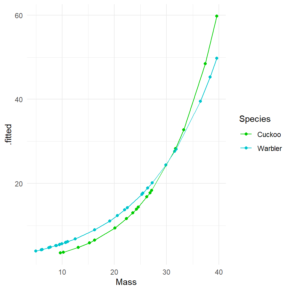
20.5.2 Log scale
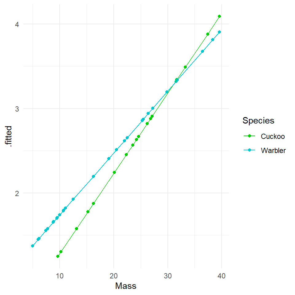
Compare the new Poisson model fits to the ordinary least squares model. We can see that although the homogeneity of variance is far from perfect, the curvature in the model has been drastically reduced (this makes sense as now we have a model fitted to exponential data), and the qqplot is within acceptable confidence intervals.
performance::check_model(cuckoo_glm1,
                         check = c("homogeneity",
                                   "qq"))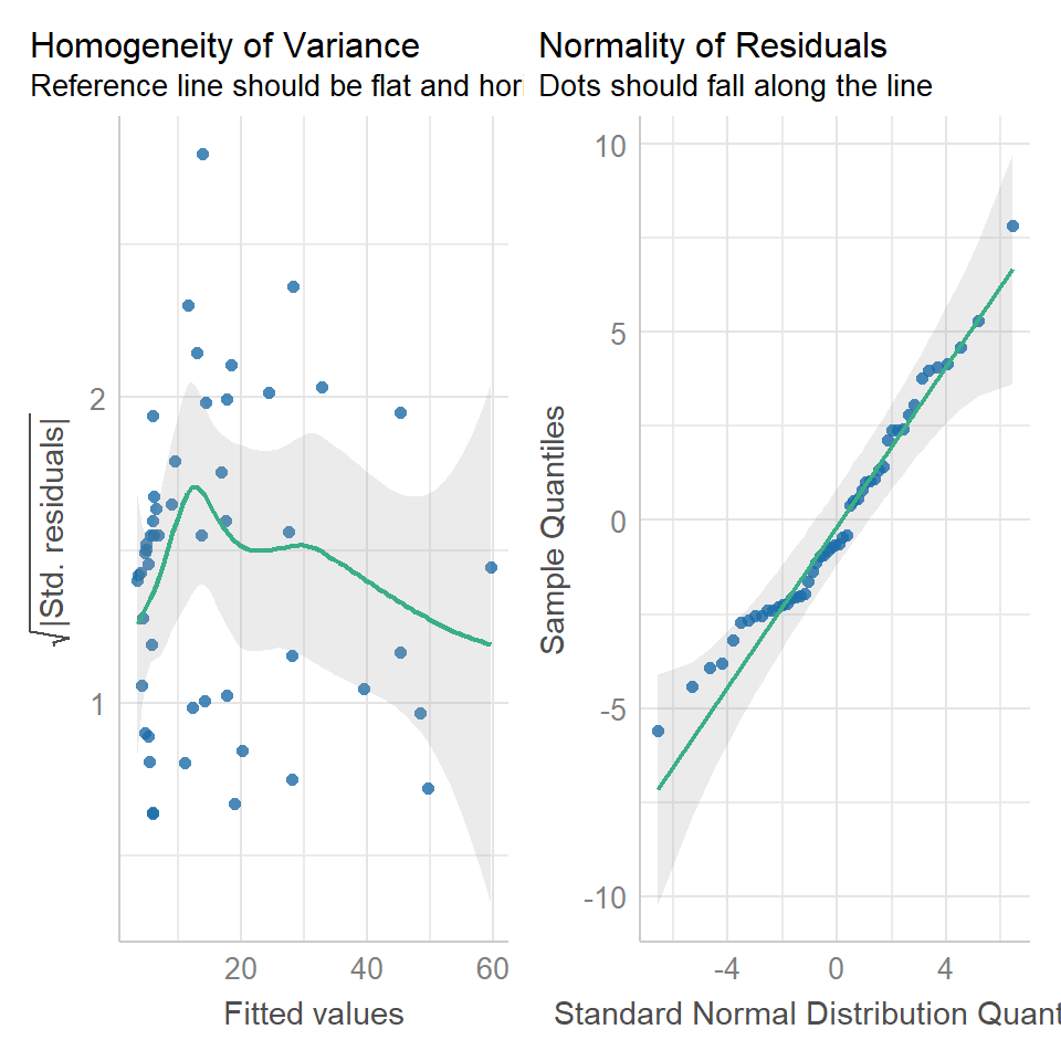
summary(cuckoo_glm1)##
## Call:
## glm(formula = Beg ~ Mass + Species + Mass:Species, family = poisson(link = "log"),
## data = cuckoo)
##
## Deviance Residuals:
## Min 1Q Median 3Q Max
## -7.5178 -2.8298 -0.6672 1.5564 6.0631
##
## Coefficients:
## Estimate Std. Error z value Pr(>|z|)
## (Intercept) 0.334475 0.227143 1.473 0.14088
## Mass 0.094847 0.007261 13.062 < 2e-16 ***
## SpeciesWarbler 0.674820 0.259217 2.603 0.00923 **
## Mass:SpeciesWarbler -0.021673 0.008389 -2.584 0.00978 **
## ---
## Signif. codes: 0 '***' 0.001 '**' 0.01 '*' 0.05 '.' 0.1 ' ' 1
##
## (Dispersion parameter for poisson family taken to be 1)
##
## Null deviance: 970.08 on 50 degrees of freedom
## Residual deviance: 436.05 on 47 degrees of freedom
## AIC: 615.83
##
## Number of Fisher Scoring iterations: 6A reminder of how to interpret the regression coefficients of a model with an interaction term
Intercept = \(\beta 0\) (intercept for the reference or baseline so here the log of the mean number of begging calls for cuckoos when mass is 0)
Mass = \(\beta1\) (slope: the change in the log mean count of begging calls for every gram of bodyweight for cuckoos)
SpeciesWarbler = \(\beta2\) (the log mean increase/decrease in begging call rate of the warblers relative to cuckoos)
Mass:SpeciesWarbler =\(\beta3\) (the log mean increase/decrease in the slope for warblers relative to cuckoos)
Because this is a Poisson distribution where variance is fixed with the mean we are using z scores. Estimates are on a log scale because of the link function - this means so are any S.E. or confidence intervals
20.6 Estimates and Intervals
Remember that not only is this Poisson model fitting variance using a Poisson and not Normal distribution. It is also relating the predictors to the response variable with a "log-link" this means we need to exponentiate our estimates to get them on the same scale as the response (y) variable. Until you do this all the model estimates are logn(y).
exp(coef(cuckoo_glm1)[1]) ### Intercept - Incidence rate at Mass=0, and Species = Cuckoo

exp(coef(cuckoo_glm1)[2]) ### Change in the average incidence rate with Mass

exp(coef(cuckoo_glm1)[3]) ### Change in the incidence rate intercept when Species = Warbler and Mass = 0

exp(coef(cuckoo_glm1)[4]) ### The extra change in incidence rate for each unit increase in Mass when Species = Warbler (the interaction effect)
## (Intercept)
## 1.397207
## Mass
## 1.09949
## SpeciesWarbler
## 1.963679
## Mass:SpeciesWarbler
## 0.9785598Luckily when you tidy your models up with broom you can specify that you want to put model predictions on the response variable scale by specifying exponentiate = T which will remove the log transformation, and allow easy calculation of confidence intervals.
broom::tidy(cuckoo_glm1,
            exponentiate = T,
conf.int = T)| term | estimate | std.error | statistic | p.value | conf.low | conf.high |
|---|---|---|---|---|---|---|
| (Intercept) | 1.3972071 | 0.2271431 | 1.472531 | 0.1408775 | 0.8858795 | 2.1589962 |
| Mass | 1.0994905 | 0.0072615 | 13.061667 | 0.0000000 | 1.0841087 | 1.1154266 |
| SpeciesWarbler | 1.9636787 | 0.2592166 | 2.603304 | 0.0092330 | 1.1889064 | 3.2864493 |
| Mass:SpeciesWarbler | 0.9785598 | 0.0083890 | -2.583559 | 0.0097787 | 0.9625068 | 0.9946969 |
20.6.1 Interpretation
It is very important to remember whether you are describing the results on the log-link scale or the original scale. It would usually make more sense to provide answers on the original scale, but this means you must first exponentiate the relationship between response predictors as described above when writing the results.
The default coefficients from the model summary are on a log scale, and are additive as such these can be added and subtracted from each other (just like ordinary least squares regression) to work out log-estimates. BUT if you exponentiate the terms of the model you get values on the 'response' scale, but these are now changes in 'rate' and are multiplicative.
Also remember that as Poisson models have 'fixed variance' z- and Chisquare distributions are used instead of t- and F.
In this example we wished to infer the relationship between begging rates and mass in these two species.
I hypothesised that the rate of begging in chicks would increase as their body size increased. Interestingly I found there was a significant interaction effect with mass and species, where Warbler chicks increased their calling rate with mass at a rate that was only 0.98 [95%CI: 0.96-0.99] that of Cuckoo chicks (Poisson GLM: \(\chi^2\)1,47 = 6.77, P = 0.009). This meant that while at hatching Warbler chicks start with a mean call rate that is higher than their parasitic brood mates, this quickly reverses as they grow.
# For a fixed  mean-variance model we use a Chisquare distribution
drop1(cuckoo_glm1, test = "Chisq")

# emmeans can be another handy function - if you specify response then here it provideds the average call rate for each species, at the average value for any continuous measures - so here the average call rate for both species at an average body mass of 20.3

emmeans::emmeans(cuckoo_glm1, specs = ~ Species:Mass, type = "response")| Df | Deviance | AIC | LRT | Pr(>Chi) | |
|---|---|---|---|---|---|
| <none> | NA | 436.0458 | 615.8282 | NA | NA |
| Mass:Species | 1 | 442.8118 | 620.5942 | 6.765991 | 0.0092911 |
##  Species Mass  rate    SE  df asymp.LCL asymp.UCL
##  Cuckoo  20.3  9.61 0.884 Inf      8.03      11.5
##  Warbler 20.3 12.15 0.658 Inf     10.93      13.5
##
## Confidence level used: 0.95
## Intervals are back-transformed from the log scale
20.7 Overdispersion
There is one extra check we need to apply to a Poisson model and that's for overdispersion
Poisson (and binomial models) assume that the variance is equal to the mean.
However, if there is residual deviance that is bigger than the residual degrees of freedom then there is more variance than we expect from the prediction of the mean by our model.
Overdispersion in Poisson models can be diagnosed by \(\frac{residual~deviance}{residual~degrees~of~freedom}\) which from our example here 'summary()' is \(\frac{436}{47} = 9.3\)
Overdispersion statistic values > 1 = Overdispersed
Overdispersion is a result of larger than expected variance for that mean under a Poisson distribution, this is clearly an issue with our model!
Luckily a simple fix is to fit a quasi-likelihood model which accounts for this, think of "quasi" as "sort of but not completely" Poisson.
cuckoo_glm2 <- glm(Beg ~ Mass+Species+Mass:Species, data=cuckoo, family=quasipoisson(link="log"))

summary(cuckoo_glm2)
##
## Call:
## glm(formula = Beg ~ Mass + Species + Mass:Species, family = quasipoisson(link = "log"),
## data = cuckoo)
##
## Deviance Residuals:
## Min 1Q Median 3Q Max
## -7.5178 -2.8298 -0.6672 1.5564 6.0631
##
## Coefficients:
## Estimate Std. Error t value Pr(>|t|)
## (Intercept) 0.33448 0.63129 0.530 0.599
## Mass 0.09485 0.02018 4.700 2.3e-05 ***
## SpeciesWarbler 0.67482 0.72043 0.937 0.354
## Mass:SpeciesWarbler -0.02167 0.02332 -0.930 0.357
## ---
## Signif. codes: 0 '***' 0.001 '**' 0.01 '*' 0.05 '.' 0.1 ' ' 1
##
## (Dispersion parameter for quasipoisson family taken to be 7.7242)
##
## Null deviance: 970.08 on 50 degrees of freedom
## Residual deviance: 436.05 on 47 degrees of freedom
## AIC: NA
##
## Number of Fisher Scoring iterations: 6As you can see, while none of the estimates have changed, the standard errors (and therefore our confidence intervals) have, this accounts for the greater than expected uncertainty we saw with the deviance, and applies a more cautious estimate of uncertainty. The interaction effect appears to no longer be significant at \(\alpha\) = 0.05, now that we have wider standard errors.
Because we are now estimating the variance again, the test statistics have reverted to t distributions and anova and drop1 functions should specify the F-test again.
20.9 Logistic regression (for binary data)
When our response variable is binary, we can use a glm with a binomial error distribution
So far we have only considered continuous and discrete data as response variables. What if our response is a categorical variable (e.g passing or failing an exam, voting yes or no in a referendum, whether an egg has successfully fledged or been predated, infected/uninfected, alive/dead)?
We can model the probability \(p\) of being in a particular class as a function of other explanatory variables.
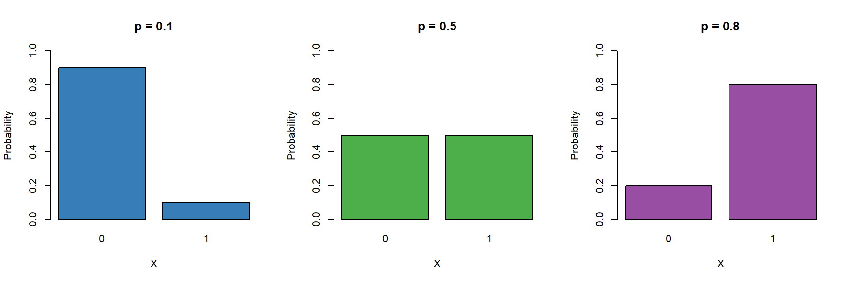
These type of binary data are assumed to follow a Bernoulli distribution (which is a special case of Binomial) which has the following characteristics:
\[ Y \sim \mathcal{Bern}(p) \]
- Binary variable, taking the values 0 or 1 (yes/no, pass/fail).
- A probability parameter \(p\), where \(0 < p < 1\).
-
Mean = \(p\)
- Variance = \(p(1 - p)\)
Let us now place the Gaussian (simple linear regression), Poisson and logistic models next to each other:
\[ \begin{aligned} Y & \sim \mathcal{N}(\mu, \sigma^2) &&& Y \sim \mathcal{Pois}(\lambda) &&& Y \sim \mathcal{Bern}(p)\\ \mu & = \beta_0 + \beta_1X &&& \log{\lambda} = \beta_0 + \beta_1X &&& ?? = \beta_0 + \beta_1X \end{aligned} \]
Now we need to fill in the ?? with the appropriate term. Similar to the Poisson regression case,
we cannot simply model the probabiliy as \(p = \beta_0 + \beta_1X\), because \(p\) cannot be negative.
\(\log{p} = \beta_0 + \beta_1X\) won't work either, because \(p\) cannot be greater than 1. Instead we
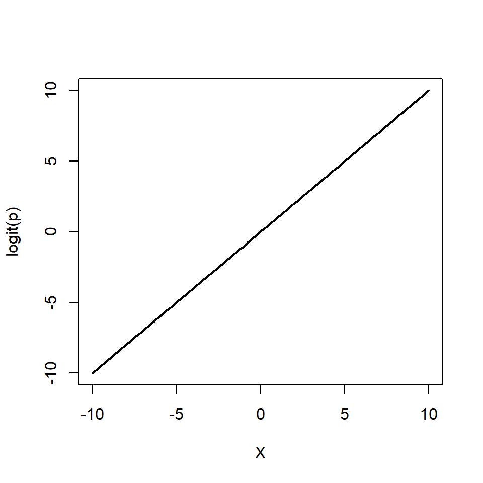
model the log odds \(\log\left(\frac{p}{1 - p}\right)\) as a linear function. So our logistic regression model looks
like this:
\[ \begin{aligned} Y & \sim \mathcal{Bern}(p)\\ \log\left(\frac{p}{1 - p}\right) & = \beta_0 + \beta_1 X \end{aligned} \]
Again, note that we are still "only" fitting straight lines through our data, but this time in the log odds space. As a shorthand notation we write \(\log\left(\frac{p}{1 - p}\right) = \text{logit}(p) = \beta_0 + \beta_1 X\).
We can also re-arrange the above equation so that we get an expression for \(p\)
\[ p = \frac{e^{\beta_0 + \beta_1 X}}{1 + e^{\beta_0 + \beta_1 X}} \]
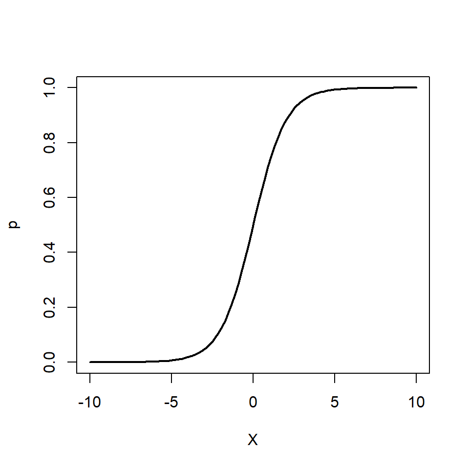
Note how \(p\) can only vary between 0 and 1.
To implement the logistic regression model in R, we choose family=binomial(link=logit) (the Bernoulli distribution is a special case of the Binomial distribution).
glm(response ~ explanatory, family=binomial(link=logit))
In 1985, NASA made the decision to send the first civilian into space.
This decision brought a huge amount of public attention to the STS-51-L mission, which would be Challenger’s 25th trip to space and school teacher Christa McAuliffe’s 1st. On the afternoon of January 28th, 1986 students around America tuned in to watch McAuliffe and six other astronauts launch from Cape Canaveral, Florida. 73 seconds into the flight, the shuttle experienced a critical failure and broke apart in mid air, resulting in the deaths of all seven crewmembers: Christa McAuliffe, Dick Scobee, Judy Resnik, Ellison Onizuka, Ronald McNair, Gregory Jarvis, and Michael Smith.
After an investigation into the incident, it was discovered that the failure was caused by an O-ring in the solid rocket booster. Additionally, it was revealed that such an incident was foreseeable.
In this half of the worksheet we will discuss how the right statistical model could have predicted the critical failure of an O-ring on that day.
head(challenger)| oring_tot | oring_dt | temp | flight |
|---|---|---|---|
| 6 | 0 | 66 | 1 |
| 6 | 1 | 70 | 2 |
| 6 | 0 | 69 | 3 |
| 6 | 0 | 68 | 4 |
| 6 | 0 | 67 | 5 |
| 6 | 0 | 72 | 6 |
The data columns are:
oring_tot: Total number of orings on the flight
oring_dt : number of orings that failed during a flight
temp: Outside temperature on the date of the flight
flight order of flights
It was frequently discussed issue that temperature might play a role in the critical safety of the o-rings on the shuttles. One of the biggest mistakes made in assessing the flight risk for the Challenger was to only look at the flights where a failure had occurred
challenger %>%
  filter(oring_dt > 0) %>%
ggplot(aes(y=oring_dt, x=temp))+geom_point()+
  ggtitle("Temperature on flight launches where an O-ring incident occurred")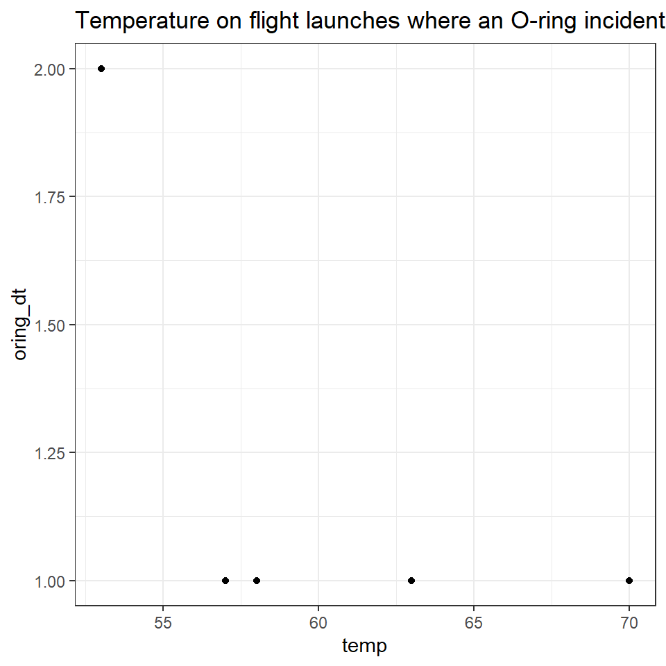
From this it was concluded that temperature did not appear to affect o-ring risk of failure, as o-ring failures were detected at a range of different temperatures.
However when we compare this to the full data that was available a very different picture emerges.
challenger %>%
ggplot(aes(y=oring_dt,
           x=temp))+
  geom_point()+
  geom_smooth(method="lm")+
  ggtitle("All launch data")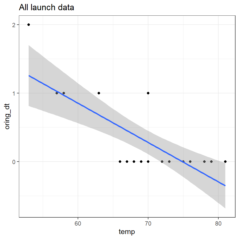
When we include the flights without incident and those with incident, we can see that there is a very clear relationship between temperature and the risk of an o-ring failure. It has been argued that the clear presentation of this data should have allowed even the casual observer to determine the high risk of disaster.
However if we want to understand the actual relationship between temperature and risk then there are several issues with fitting a linear model here - once again the data is an integer, and bounded by zero (our model predicts negative failure rates within the observed data range).
We COULD consider this as suitable for a Poisson model - but if we are really interested in determining the binary risk of having a flight with o-ring failure vs. no failure. Then we should implement a GLM with a Binomial distribution.
We can use dplyr to generate a binary column of no incident '0' and fail '1' for anything >0.
Fitting a binary GLM
binary_model <- glm(oring_binary~temp, family=binomial, data=challenger)
binary_model %>%
broom::tidy(conf.int=T)| term | estimate | std.error | statistic | p.value | conf.low | conf.high |
|---|---|---|---|---|---|---|
| (Intercept) | 23.7749552 | 11.8203514 | 2.011358 | 0.0442877 | 7.2430347 | 58.1947978 |
| temp | -0.3667009 | 0.1751673 | -2.093432 | 0.0363106 | -0.8772585 | -0.1217173 |
So we are now fitting the following model
\[ Y \sim Bern(p) \] \[ \log\left[ \frac { P( \operatorname{oring\_binary} = fail) }{ 1 - P( \operatorname{oring\_binary} = fail) } \right] = \beta_{0} + \beta_{1}(\operatorname{temp}) \]
Which in R will look like this:
binary_model <- glm(oring_binary~temp, family=binomial, data=challenger)- Intercept = \(\beta_{0}\) = 23.77
When the temperature is 0°F the mean log-odds are 23.77 [95%CI: 7.24- 58.19] for a failure incident in the O-rings
- Temp = \(\beta_{1}\) = -0.37 [95%CI: -0.87 - -0.12]
For every rise in the temperature by 1°F, the log-odds of a critical incident fall by 0.37.
20.9.1 Interpreting model coefficients
We first consider why we are dealing with odds \(\frac{p}{1-p}\) instead of just \(p\). They contain the same information, so the choice is somewhat arbitrary, however we’ve been using probabilities for so long that it feels unnatural to switch to odds. There are good reasons for this, however. Odds \(\frac{p}{1-p}\) can take on any value from 0 to ∞ and so part of our translation of \(p\) to an unrestricted domain is already done (\(P\) is restricted to 0-1). Take a look at some examples below:
| Probability | Odds | Verbiage |
|---|---|---|
| \(p=.95\) | \(\frac{95}{5} = \frac{19}{1} = 19\) | 19 to 1 odds for |
| \(p=.75\) | \(\frac{75}{25} = \frac{3}{1} = 3\) | 3 to 1 odds for |
| \(p=.50\) | \(\frac{50}{50} = \frac{1}{1} = 1\) | 1 to 1 odds |
| \(p=.25\) | \(\frac{25}{75} = \frac{1}{3} = 0.33\) | 3 to 1 odds against |
| \(p=.05\) | \(\frac{95}{5} = \frac{1}{19} = 0.0526\) | 19 to 1 odds against |
When we use a binomial model, we produce the 'log-odds', this produces a fully unconstrained linear regression as anything less than 1, can now occupy an infinite negative value -∞ to ∞.
\[\log\left(\frac{p}{1-p}\right) = \beta_{0}+\beta_{1}x_{1}+\beta_{2}x_{2} \]
\[\frac{p}{1-p} = e^{\beta_{0}}e^{\beta_{1}x_{1}}e^{\beta_{2}x_{2}} \]
We can interpret \(\beta_{1}\) and \(\beta_{2}\) as the increase in the log odds for every unit increase in \(x_{1}\) and \(x_{2}\). We could alternatively interpret \(\beta_{1}\) and \(\beta_{2}\) using the notion that a one unit change in \(x_{1}\) as a percent change of \(e^{\beta_{1}}\) in the odds. That is to say, \(e^{\beta_{1}}\) is the odds ratio of that change.
If you want to find out more about Odds and log-odds head here
20.10 Probability
A powerful use of logisitic regression is prediction. Can we predict the probability of an event occuring using our data?
20.10.1 Activity 3: Make predictions
Can you use our prediction functions predict() or broom::augment() to look at the models predictions for O-ring failure in our data? Bonus points if you can convert log-odds to probability?
20.10.2 Emmeans
If we use the emmeans() function it will convert log-odds to estimate the probability of o-ring failure at the mean value of x (temperature). And add confidence intervals!
But how do log-odds and probability actually relate?
emmeans::emmeans(binary_model, specs=~temp, type="response")## temp prob SE df asymp.LCL asymp.UCL
## 69.6 0.15 0.0985 Inf 0.0373 0.445
##
## Confidence level used: 0.95
## Intervals are back-transformed from the logit scaleThis is the equation to work out probability using the exponent of the linear regression equation:
\[ P(\operatorname{risk of failure at } X=69)\left[ \frac{e^{23.77+(-0.37 \times 69.6)}}{1+e^{23.77+(-0.37 \times 69.6)}} \right] \]
Which produces the following result and we can confirm the risk of an o-ring failure on an average day is 0.15
odds_at_69.6 <- exp(coef(binary_model)[1]+coef(binary_model)[2]*69.6)
# To convert from odds to a probability, divide the odds by one plus the odds

probability <-  odds_at_69.6/(1+odds_at_69.6)
probability
## (Intercept)
## 0.148371720.10.3 Changes in probability
A useful rule-of-thumb can be the divide-by-four rule.
This can be described as the maximum difference in probability for a unit change in \(X\) is \(\beta/4\).
In our example the maximum difference in probability from a one degree change in Temp is \(-0.37/4 = -0.09\)
So the maximum difference in probability of failure corresponding to a one degree change is 9%
Remember if you want to augment your data with the model, you can use the augment() function, remembering to specify type.predict = "response to get probabilities of o-ring failure (not log odds).
| oring_binary | temp | .fitted | .se.fit | .resid | .std.resid | .hat | .sigma | .cooksd |
|---|---|---|---|---|---|---|---|---|
| 0 | 66 | 0.3947697 | 0.1701810 | -1.0021439 | -1.0690274 | 0.1212153 | 0.8149531 | 0.0511900 |
| 1 | 70 | 0.1307765 | 0.0924586 | 2.0170599 | 2.0974690 | 0.0752029 | 0.7080401 | 0.2922222 |
| 0 | 69 | 0.1783731 | 0.1067906 | -0.6268474 | -0.6527589 | 0.0778149 | 0.8366510 | 0.0099323 |
| 0 | 68 | 0.2385386 | 0.1234222 | -0.7382625 | -0.7713137 | 0.0838649 | 0.8315908 | 0.0156510 |
| 0 | 67 | 0.3113088 | 0.1444333 | -0.8636693 | -0.9090255 | 0.0973013 | 0.8246049 | 0.0269880 |
| 0 | 72 | 0.0673886 | 0.0661208 | -0.3735417 | -0.3872542 | 0.0695651 | 0.8448617 | 0.0029032 |
Annoyingly a limitation of the augment function is that it won't produce 95% CI for predictions on glms. But I have written a short function to do this Don't worry if this is a lot to get your head around - the main thing is use this code to produce 95% CI.
augment_glm <- function(mod, predict = NULL){
  fam <- family(mod)
  ilink <- fam$linkinv

  broom::augment(mod, newdata = predict, se_fit=T)%>%
    mutate(.lower = ilink(.fitted - 1.96*.se.fit),
           .upper = ilink(.fitted + 1.96*.se.fit),
           .fitted=ilink(.fitted))
}

augment_glm(binary_model)| oring_binary | temp | .fitted | .se.fit | .resid | .std.resid | .hat | .sigma | .cooksd | .lower | .upper |
|---|---|---|---|---|---|---|---|---|---|---|
| 0 | 66 | 0.3947697 | 0.7122731 | -1.0021439 | -1.0690274 | 0.1212153 | 0.8149531 | 0.0511900 | 0.1390310 | 0.7248700 |
| 1 | 70 | 0.1307765 | 0.8133661 | 2.0170599 | 2.0974690 | 0.0752029 | 0.7080401 | 0.2922222 | 0.0296467 | 0.4255788 |
| 0 | 69 | 0.1783731 | 0.7286671 | -0.6268474 | -0.6527589 | 0.0778149 | 0.8366510 | 0.0099323 | 0.0494727 | 0.4752149 |
| 0 | 68 | 0.2385386 | 0.6794956 | -0.7382625 | -0.7713137 | 0.0838649 | 0.8315908 | 0.0156510 | 0.0763842 | 0.5426717 |
| 0 | 67 | 0.3113088 | 0.6736765 | -0.8636693 | -0.9090255 | 0.0973013 | 0.8246049 | 0.0269880 | 0.1077038 | 0.6286427 |
| 0 | 72 | 0.0673886 | 1.0520852 | -0.3735417 | -0.3872542 | 0.0695651 | 0.8448617 | 0.0029032 | 0.0091067 | 0.3622931 |
| 0 | 73 | 0.0476880 | 1.1923059 | -0.3126102 | -0.3232178 | 0.0645605 | 0.8462069 | 0.0018473 | 0.0048153 | 0.3413479 |
| 0 | 70 | 0.1307765 | 0.8133661 | -0.5294432 | -0.5505492 | 0.0752029 | 0.8403180 | 0.0066147 | 0.0296467 | 0.4255788 |
| 1 | 57 | 0.9464956 | 1.9365672 | 0.3316293 | 0.3684596 | 0.1899238 | 0.8452819 | 0.0081803 | 0.2844142 | 0.9987315 |
| 1 | 63 | 0.6621290 | 1.0178481 | 0.9080692 | 1.0360335 | 0.2317717 | 0.8170810 | 0.1001978 | 0.2104548 | 0.9350983 |
| 1 | 70 | 0.1307765 | 0.8133661 | 2.0170599 | 2.0974690 | 0.0752029 | 0.7080401 | 0.2922222 | 0.0296467 | 0.4255788 |
| 0 | 78 | 0.0079412 | 1.9788007 | -0.1262767 | -0.1282707 | 0.0308485 | 0.8488032 | 0.0001315 | 0.0001655 | 0.2790320 |
| 0 | 67 | 0.3113088 | 0.6736765 | -0.8636693 | -0.9090255 | 0.0973013 | 0.8246049 | 0.0269880 | 0.1077038 | 0.6286427 |
| 1 | 53 | 0.9871288 | 2.6052168 | 0.1609645 | 0.1683888 | 0.0862364 | 0.8484526 | 0.0006733 | 0.3172542 | 0.9999210 |
| 0 | 67 | 0.3113088 | 0.6736765 | -0.8636693 | -0.9090255 | 0.0973013 | 0.8246049 | 0.0269880 | 0.1077038 | 0.6286427 |
| 0 | 75 | 0.0234853 | 1.4950302 | -0.2180160 | -0.2238281 | 0.0512601 | 0.8478117 | 0.0006848 | 0.0012822 | 0.3105914 |
| 0 | 70 | 0.1307765 | 0.8133661 | -0.5294432 | -0.5505492 | 0.0752029 | 0.8403180 | 0.0066147 | 0.0296467 | 0.4255788 |
| 0 | 81 | 0.0026572 | 2.4796156 | -0.0729485 | -0.0735502 | 0.0162947 | 0.8491284 | 0.0000224 | 0.0000206 | 0.2558266 |
| 0 | 76 | 0.0163939 | 1.6534591 | -0.1818228 | -0.1859683 | 0.0440855 | 0.8482690 | 0.0004021 | 0.0006518 | 0.2986916 |
| 0 | 79 | 0.0055168 | 2.1444266 | -0.1051866 | -0.1065392 | 0.0252300 | 0.8489535 | 0.0000737 | 0.0000829 | 0.2706470 |
| 0 | 75 | 0.0234853 | 1.4950302 | -0.2180160 | -0.2238281 | 0.0512601 | 0.8478117 | 0.0006848 | 0.0012822 | 0.3105914 |
| 0 | 76 | 0.0163939 | 1.6534591 | -0.1818228 | -0.1859683 | 0.0440855 | 0.8482690 | 0.0004021 | 0.0006518 | 0.2986916 |
| 1 | 58 | 0.9245824 | 1.7732723 | 0.3960130 | 0.4481860 | 0.2192676 | 0.8433540 | 0.0146713 | 0.2750175 | 0.9974824 |
Alternatively we can also do this calculation via emmeans
##  temp     prob         SE  df asymp.LCL asymp.UCL
##    66 0.394770 0.17018097 Inf  0.139034  0.724865
##    65 0.484853 0.19701707 Inf  0.167060  0.815387
##    64 0.575932 0.21823406 Inf  0.190739  0.886694
##    63 0.662129 0.22770706 Inf  0.210461  0.935096
##    62 0.738753 0.22299102 Inf  0.227046  0.964568
##    61 0.803166 0.20584013 Inf  0.241266  0.981259
##    60 0.854818 0.18057075 Inf  0.253727  0.990288
##    59 0.894693 0.15192302 Inf  0.264874  0.995033
##    58 0.924582 0.12364996 Inf  0.275030  0.997482
##    57 0.946496 0.09807106 Inf  0.284428  0.998731
##    56 0.962301 0.07624709 Inf  0.293240  0.999364
##    55 0.973568 0.05837488 Inf  0.301592  0.999682
##    54 0.981533 0.04416262 Inf  0.309579  0.999841
##    53 0.987129 0.03310075 Inf  0.317275  0.999921
##    52 0.991045 0.02462725 Inf  0.324734  0.999961
##    51 0.993777 0.01821445 Inf  0.332003  0.999981
##    50 0.995679 0.01340624 Inf  0.339114  0.999990
##    49 0.997001 0.00982751 Inf  0.346096  0.999995
##    48 0.997920 0.00717951 Inf  0.352970  0.999998
##    47 0.998558 0.00522962 Inf  0.359755  0.999999
##    46 0.999000 0.00379955 Inf  0.366464  0.999999
##    45 0.999307 0.00275431 Inf  0.373111  1.000000
##    44 0.999520 0.00199257 Inf  0.379705  1.000000
##    43 0.999667 0.00143888 Inf  0.386253  1.000000
##    42 0.999769 0.00103733 Inf  0.392763  1.000000
##    41 0.999840 0.00074671 Inf  0.399239  1.000000
##    40 0.999889 0.00053676 Inf  0.405687  1.000000
##    39 0.999923 0.00038534 Inf  0.412110  1.000000
##    38 0.999947 0.00027631 Inf  0.418510  1.000000
##    37 0.999963 0.00019791 Inf  0.424891  1.000000
##    36 0.999974 0.00014160 Inf  0.431253  1.000000
##    35 0.999982 0.00010122 Inf  0.437600  1.000000
##    34 0.999988 0.00007228 Inf  0.443931  1.000000
##    33 0.999992 0.00005158 Inf  0.450247  1.000000
##    32 0.999994 0.00003677 Inf  0.456549  1.000000
##    31 0.999996 0.00002619 Inf  0.462837  1.000000
##    30 0.999997 0.00001865 Inf  0.469112  1.000000
##    29 0.999998 0.00001327 Inf  0.475372  1.000000
##    28 0.999999 0.00000943 Inf  0.481619  1.000000
##    27 0.999999 0.00000670 Inf  0.487850  1.000000
##
## Confidence level used: 0.95
## Intervals are back-transformed from the logit scale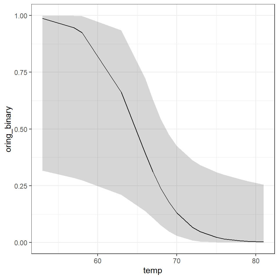
20.11 Predictions
On the day the Challenger launched the outside air temperature was 36°F
We can use augment to add our model to new data - and make predictions about the risk of o-ring failure
20.12 Assumptions
The standard model checks from plot() cannot be used on binomial glms, they are usually a mess!
Luckily the performance package detects and alters the checks. Pay particular attention to the binned residuals plot - this is your best estimate of possible overdispersion (requiring a quasi-likelihood check). In this case there is likely not enough data for robust checks
performance::check_model(binary_model)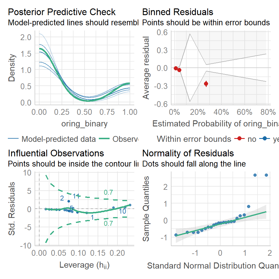
20.12.1 Activity 5: Write-up
How would you write up for findings from this analysis?
Analysis: I used a Binomial logit-link Generalized Linear Model to analyse the effect of temperature on the likelihood of O-ring failure.
All analyses were carried out in R (ver 4.1.3) (R Core Team 2021) with the following packages; tidyverse (Wickham et al 2019).
Results: I found a significant negative relationship between temperature and probability of o-ring failure (logit-odds = -0.37 [95%CI: -0.88 - -0.12], z = -2.1, d.f = 21, P = 0.036). At an average temperature of 69.6°F the probability of o-ring failure was estimated at 0.15[0.03-0.45], but this rose to a near certainty of failure 0.99[0.43-1] at 36°F.
Note you could use drop1( test = "Chisq") here, but as there is only one, continuous variable, we can also report directly from the summary table.
drop1(binary_model, test="Chisq")| Df | Deviance | AIC | LRT | Pr(>Chi) | |
|---|---|---|---|---|---|
| <none> | NA | 14.42579 | 18.42579 | NA | NA |
| temp | 1 | 26.40237 | 28.40237 | 11.97658 | 0.0005387 |
20.13 Summary
GLMs are powerful and flexible.
They can be used to fit a wide variety of data types.
Model checking becomes trickier.
Extensions include:
- mixed models;
- survival models;
- generalized additive models (GAMs).
For more information on Poisson and Binomial GLMs check out:
https://bookdown.org/dereksonderegger/571/11-binomial-regression.html#confidence-intervals-1
https://bookdown.org/ronsarafian/IntrotoDS/glm.html#poisson-regression
20.14 Final checklist
Think carefully about the hypotheses to test, use your scientific knowledge and background reading to support this
Import, clean and understand your dataset: use data visuals to investigate trends and determine if there is clear support for your hypotheses
Decide on the appropriate error structure for your model (Gaussian = continuous, Poisson = count, Binomial = binary)
Start with canonical link functions, but these can be altered if needed
Fit a (generalized) linear model, including interaction terms with caution
Investigate the fit of your model, understand that parameters may never be perfect, but that classic patterns in residuals may indicate a poorly fitting model - sometimes this can be fixed with careful consideration of missing variables or through data transformation
Check for overdispersion in models where variance is not estimated independently of the mean (Poisson and Binomial) - may have to use quasi-likelihood fitting
Test the removal of any interaction terms from a model, look at AIC and significance tests (Remember test = "F" for Gaussian and Quasilikelihood models, "Chisq" for Poisson and Binomial models)
Make sure you understand the output of a model summary, sense check this against the graphs you have made - Do estimates need converting back to the original response scale?
The direction and size of any effects are the priority - produce estimates and uncertainties. Make sure the observations are clear.
Write-up your significance test results, taking care to report not just significance (and all required parts of a significance test). Do you know what to report? Within a complex model - reporting t/z will indicate the slope of the line for that single term against the intercept, F/Chi is the overall effect of a predictor across all levels, post-hoc if you wish to compare across all levels.
Well described tables and figures can enhance your results sections - take the time to make sure these are informative and attractive.