library(tidyverse)
library(here)
library(rstatix)     # simple t-tests with tidy output
library(broom)       # tidy model summaries (optional)
library(sandwich)    # robust (heteroskedasticity-consistent) variance estimators
library(lmtest)      # coeftest/coefci for robust inference
library(performance) # easy model checks8 Linear models and t-tests
In the last chapter we analyzed Darwin’s maize data and computed confidence intervals “by hand.” That helped build intuition about estimates, standard errors, and confidence. Here, we’ll move to faster, standard tools:
-
rstatix::t_test()for two-sample t-tests (Welch and equal-variance/Student). -
lm()for linear models (which also reproduces the two-sample t-test). -
lm()withsandwich(robust) standard errors to guard against unequal variances.
8.0.1 Packages
8.1 Quick start: two-sample t-tests with rstatix
The function rstatix::t_test() conducts a two-sample t-test from a simple formula: outcome ~ group.
Welch’s t-test (default; does not assume equal variances)
Student’s t-test (set
var.equal = TRUEto assume equal variances)
| estimate | estimate1 | estimate2 | .y. | group1 | group2 | n1 | n2 | statistic | p | df | conf.low | conf.high | method | alternative |
|---|---|---|---|---|---|---|---|---|---|---|---|---|---|---|
| 2.616667 | 20.19167 | 17.575 | height | Cross | Self | 15 | 15 | 2.437113 | 0.0233 | 22.16409 | 0.3909566 | 4.842377 | T-test | two.sided |
| estimate | estimate1 | estimate2 | .y. | group1 | group2 | n1 | n2 | statistic | p | df | conf.low | conf.high | method | alternative |
|---|---|---|---|---|---|---|---|---|---|---|---|---|---|---|
| 2.616667 | 20.19167 | 17.575 | height | Cross | Self | 15 | 15 | 2.437113 | 0.0214 | 28 | 0.4173433 | 4.81599 | T-test | two.sided |
The core outputs are:
estimate: the difference in means (reference group is the first level in alphabetical order unless otherwise set)
conf.low, conf.high: 95% confidence interval
statistic, df, p: t-value, degrees of freedom, and p-value
You can also quickly see group summaries:
| type | n | mean | sd | se |
|---|---|---|---|---|
| Cross | 15 | 20.19167 | 3.616945 | 0.9338912 |
| Self | 15 | 17.57500 | 2.051676 | 0.5297405 |
Tip
Which t-test should I use? - Start with Welch (default), as it is robust to unequal variances. - If you have good reason (and checks) to assume equal variances, use var.equal = TRUE.
Note
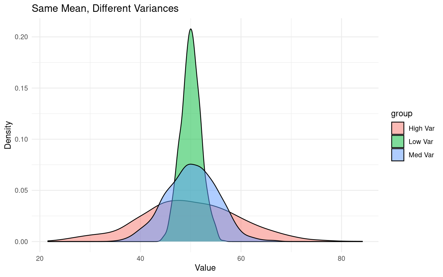
NoteWhat is variance?
Variance is a statistical measure of how spread out or dispersed a dataset is from its mean. Student vs Welch’s t use two different calculations that either “pool” or keep sd separate when comparing group means:
8.2 A linear model (lm) approach
A two-sample t-test is a special case of a linear model. With lm(height ~ type), the coefficient for the non-reference level represents the difference in means. Most of the common statistical models (t-test, correlation, ANOVA; chi-square, etc.) are special cases of linear models or a very close approximation. This beautiful simplicity means that there is less to learn:
The linear-model uses a technique called least squares.
8.3 Summaries for models
When you have made a linear model, we can investigate a summary of the model using the base R function summary(). There is also a tidyverse option provided by the package broom(Robinson et al. (2024)).
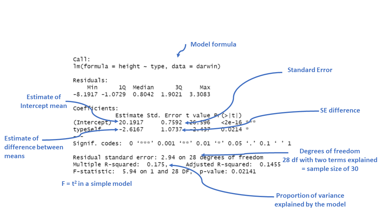
Call:
lm(formula = height ~ type, data = darwin)

Residuals:
    Min      1Q  Median      3Q     Max
-8.1917 -1.0729  0.8042  1.9021  3.3083

Coefficients:
            Estimate Std. Error t value Pr(>|t|)
(Intercept)  20.1917     0.7592  26.596   <2e-16 ***
typeSelf     -2.6167     1.0737  -2.437   0.0214 *
---
Signif. codes:  0 '***' 0.001 '**' 0.01 '*' 0.05 '.' 0.1 ' ' 1

Residual standard error: 2.94 on 28 degrees of freedom
Multiple R-squared:  0.175, Adjusted R-squared:  0.1455
F-statistic: 5.94 on 1 and 28 DF, p-value: 0.02141Key interpretations:
-
Intercept: mean height of the reference level of
type(the first level of the factor).This is the predicted height when the plant type is “Cross” fertilised, which is the reference category). The estimate is 20.1917, which means the average height for plants that are not self-fertilised is about 20.19 inches.
-
typeSelf (for example): estimated difference in means between Self and the reference (e.g., Cross). A negative value means Self is shorter on average.
typeSelf: This coefficient tells us how the height of “Self” fertilized plants differs from the reference group (“Cross” fertilized plants). The estimate is -2.6167, meaning “Self” fertilized plants are, on average, 2.62 units shorter than “Cross” fertilized plants.
To confirm the reference level and means:
NULL| type | mean |
|---|---|
| Cross | 20.19167 |
| Self | 17.57500 |
NoteMore information on model summaries
The Std. Error for each coefficient measures the uncertainty in the estimate. Smaller values indicate more precise estimates. For example, the standard error of 1.0737 for the “typeSelf” coefficient suggests there’s some variability in how much shorter the “Self” fertilized plants are, but it’s reasonably precise.
The t value is the ratio of the estimate to its standard error (\(\frac{Mean}{Std. Error}\)). The larger the t-value (either positive or negative), the more evidence there is that the estimate is different from zero.
Pr(>|t|) gives the p-value, which tells us the probability of observing a result as extreme as this, assuming that there is no real effect (i.e., the null hypothesis is true). In this case, a p-value of 0.0214 means there’s about a 2% chance that the difference in height between “Self” and “Cross” fertilized plants is due to random chance. Since this is below the typical cutoff of 0.05, it suggests that the difference is statistically significant.
Significance codes: These symbols next to the p-value indicate how strong the evidence is. In this case, one star (*) indicates a p-value below 0.05, meaning the effect is considered statistically significant.
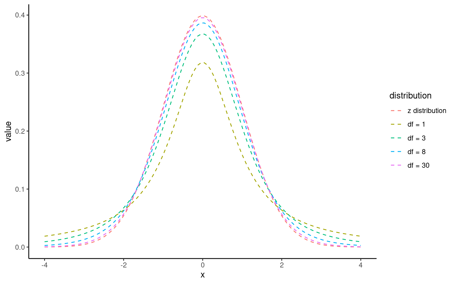
The t-distribution looks like a normal distribution but with heavier tails for small samples.
As sample size grows, it approaches the normal distribution.
8.3.1 The t-Distribution:
The t-distribution is similar to the normal distribution but has more spread (wider tails), especially with smaller sample sizes. As the sample size increases, the t-distribution approaches the normal distribution.
NoteA simple write up
From this summary model we can make conclusions about the effect of inbreeding and produce a simple write up:
“The maize plants that have been cross pollinated had an average height (mean ±S.E.) of 20.19 (± 0.76) inches and were taller on average than the self-pollinated plants, with a mean difference in height of 2.62 (±1.07) inches (t(28) = -2.44, p = 0.02)”
8.4 Confidence intervals
8.4.1 What a 95% confidence interval means
A 95% confidence interval (CI) gives a plausible range for the true effect in the population (e.g., the true difference in mean height between Cross and Self).
If we repeated the same study many times and built a 95% CI each time, about 95% of those intervals would contain the true effect.
Narrow CIs = more precision (usually larger sample size or less variability). Wide CIs = more uncertainty.
8.4.2 Why you should always report CIs
A p-value is a single number about “is there evidence of an effect?” but does not tell you “how big might the effect be?”.
A CI shows both the estimated effect size and the uncertainty around it. Always report your estimate with its 95% CI.
Example (difference in means):
Mean difference = 2.62 inches, 95% CI [0.42, 4.82]
Interpretation: The true difference is plausibly between 0.42 and 4.82 inches; values near 0 are less compatible with the data than values around 2–3 inches.
NoteHow CIs and p-values relate (two-sided tests)
For a two-sided test at α = 0.05, a 95% CI that does not include 0 corresponds to p < 0.05 (statistically significant).
If the 95% CI includes 0, then p ≥ 0.05 (not statistically significant).
This is why CIs are often described as the “interval version” of the p-value decision.
Tip: - For the question “Is there a difference?”, look at the 95% CI for the difference. If it excludes 0, there is evidence of a difference.
- Be careful with overlapping CIs on separate group means: overlapping mean CIs do not necessarily imply “no difference.” The definitive check is the CI for the difference itself.
8.4.3 What changes CI width?
Sample size: larger n → narrower CI.
Variability: more spread in data → wider CI.
Confidence level: 99% CI is wider than 95% CI (stricter evidence requirement).
8.4.4 How to report (templates)
Difference: “The mean difference was X [95% CI: L, U].”
Group means: “Cross mean = A [95% CI: L1, U1]; Self mean = B [95% CI: L2, U2].”
Match the CI to your method (Welch, equal-variance, or robust SE) and keep the reporting consistent.
8.4.5 Confidence intervals (CI) in R
With a wrapper function around our model we can generate accurate 95% confidence intervals from the SE and calculated t-distribution:
Because this follows the same layout as the table of coefficients, the output intercept row gives a 95% CI for the height of the crossed plants and the second row gives a 95% interval for the difference in height between crossed and selfed plants. The lower and upper bounds are the 2.5% and 97.5% of a t-distribution.
It is this difference in height in which we are specifically interested.
8.5 Robust standard errors with sandwich
When we were first introduced to the t-test we learned about Student’s (equal variance) vs Welch’s test (unequal variance).
If variances differ across groups (heteroscedasticity), standard errors from lm() may be too optimistic (like the student’s t-test). A simple fix is to use heteroskedasticity-consistent (HC) “sandwich” standard errors (like Welch’s t-test).
# Fit the same model
lsmodel1 <- lm(height ~ type, data = darwin)

# Robust (HC3) SEs and tests for coefficients
lmtest::coeftest(lsmodel1, vcov. = sandwich::vcovHC(lsmodel1, type = "HC3"))

# Robust confidence intervals for coefficients
lmtest::coefci(lsmodel1, vcov. = sandwich::vcovHC(lsmodel1, type = "HC3"), level = 0.95)
t test of coefficients:

            Estimate Std. Error t value Pr(>|t|)
(Intercept) 20.19167    0.96667 20.8879  < 2e-16 ***
typeSelf    -2.61667    1.11136 -2.3545  0.02579 *
---
Signif. codes:  0 '***' 0.001 '**' 0.01 '*' 0.05 '.' 0.1 ' ' 1

                2.5 %     97.5 %
(Intercept) 18.211535 22.1717988
typeSelf    -4.893183 -0.3401508
Interpretation: - The coefficient for typeSelf is still the difference in means, but its SE, t, p, and CI are now robust to unequal variances.
- Use this when Levene’s test (or model check plots) suggest heteroscedasticity, or as a cautious default.
Note
sandwich::vcovHC()computes a heteroskedasticity-consistent covariance matrix.“HC3” is often preferred (like in MacKinnon & White, 1985) because it’s more reliable in small samples.
lmtest::coeftest()replaces the usual OLS standard errors with these robust ones.lmtest::coefci()gives robust CIs with the same robust covariance matrix.
8.6 Assumptions: minimal, practical checks
When we fit a linear model for a two-group comparison, we need to check whether the numbers we have generated are reliable by checking the fit of our model against some assumptions:
Normality: The t-test and lm are fairly robust for moderate sample sizes. A quick check is still useful.
Equal variances: Prefer Welch or robust SEs if this looks violated.
Making these checks is simple and quick with performance::check_model()
# -------------------------------------------------------------------
# Check the NORMALITY of residuals for the linear model 'lsmodel1'
# -------------------------------------------------------------------
# Purpose:
# - In linear regression, residuals should ideally be normally distributed.
# This affects the validity of confidence intervals and p-values.
normality <- check_normality(lsmodel1)
# Print the results of the normality test.
# The output will usually include:
# - The type of test used ("Shapiro-Wilk")
# Interpretation:
# - p > 0.05 → Fail to reject normality (residuals are approximately normal)
# - p < 0.05 → Reject normality (residuals deviate from normality)
normality
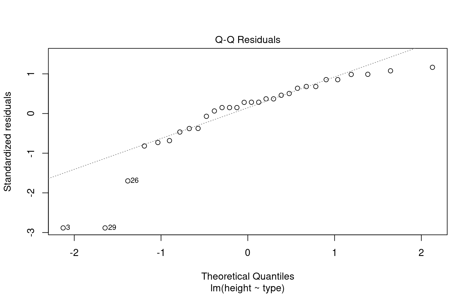
# Visualize the normality check with a Q–Q plot (quantile–quantile plot).
#
# The plot() method for the object returned by 'check_normality()' creates:
# - A Q–Q plot comparing the quantiles of the residuals
# against the theoretical quantiles from a normal distribution.
# - The line represents the "ideal" normal distribution.
# Argument:
# detrend = FALSE → Shows the standard Q–Q plot (not detrended).
# If TRUE, it shows the residuals from the Q–Q line (useful for subtle deviations).
#
# Interpretation:
# - Points should roughly follow the diagonal line.
# - Systematic deviations (S-shaped curve or tails off the line)
# indicate non-normal residuals.
plot(normality, detrend = FALSE)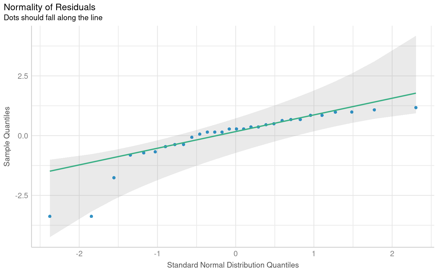
# -------------------------------------------------------------------
# Check for HETEROSCEDASTICITY (unequal variances of residuals)
# -------------------------------------------------------------------
# The function 'check_heteroscedasticity()' tests whether the residuals
# from the model have constant variance (homoscedasticity).
#
# Under the hood, it typically performs:
# - Breusch–Pagan test (default)
#
# Purpose:
# - In linear regression, we assume the variance of residuals is constant
# across fitted values (homoscedasticity).
# - Heteroscedasticity can bias standard errors and affect inference.
heteroscedasticity <- check_heteroscedasticity(lsmodel1)
# Print the test results.
# Output typically includes:
# - The type of test used (usually "Breusch–Pagan")
# Interpretation:
# - p > 0.05 → No evidence of heteroscedasticity (good)
# - p < 0.05 → Residual variance changes with fitted values (problematic)
heteroscedasticity
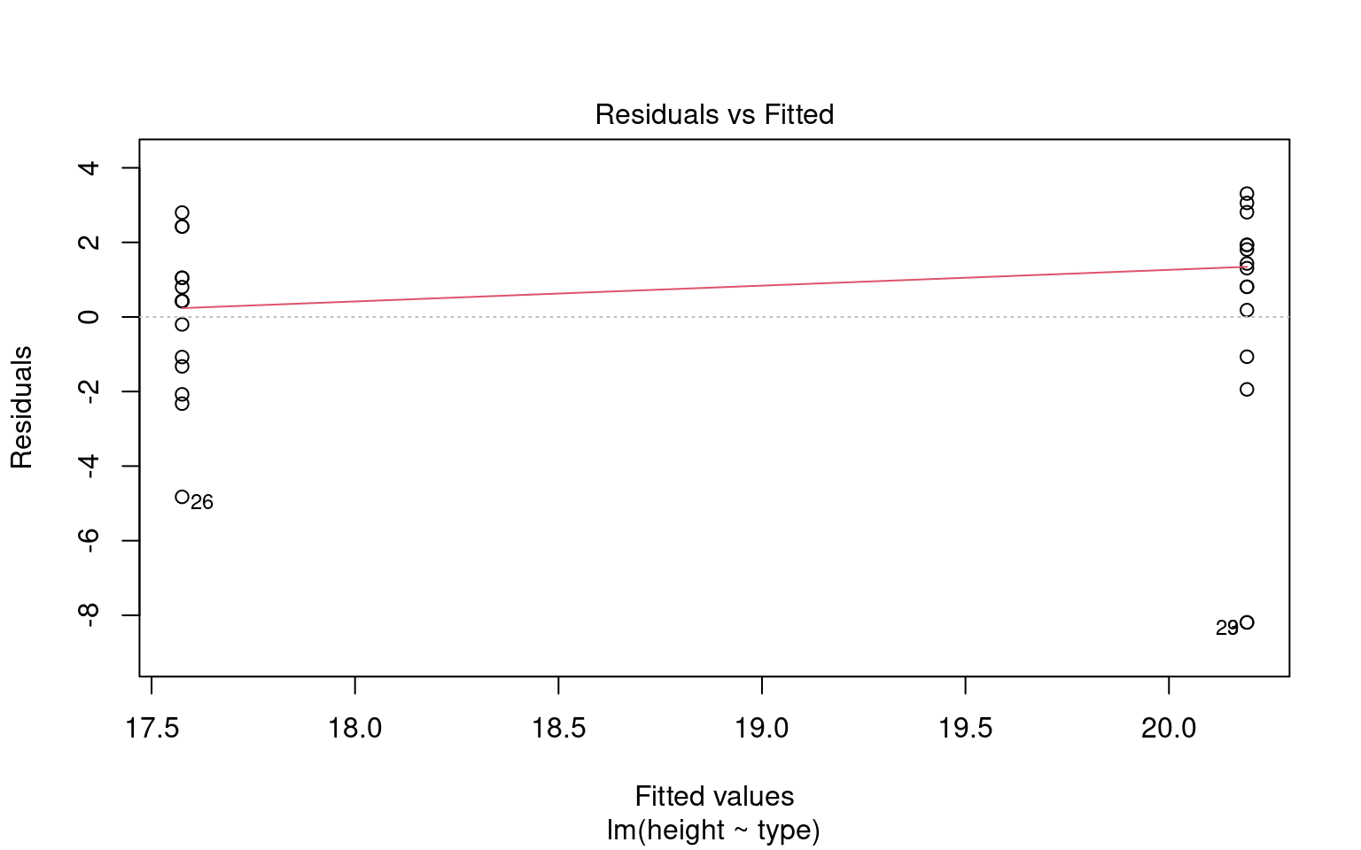
# Visualize the results with a residuals-vs-fitted plot.
# The plot() method for 'check_heteroscedasticity()' creates:
# - A scatterplot of fitted values (x-axis) vs. residuals (y-axis)
# - A smoothing line (usually loess) that helps detect trends.
#
# Interpretation:
# - Random scatter around zero → Homoscedasticity (good)
# - Funnel shape or systematic pattern → Heteroscedasticity (bad)
# Unfortunately this plot is a BIT RUBBISH when comparing groups - check out the basic R function instead
plot(heteroscedasticity)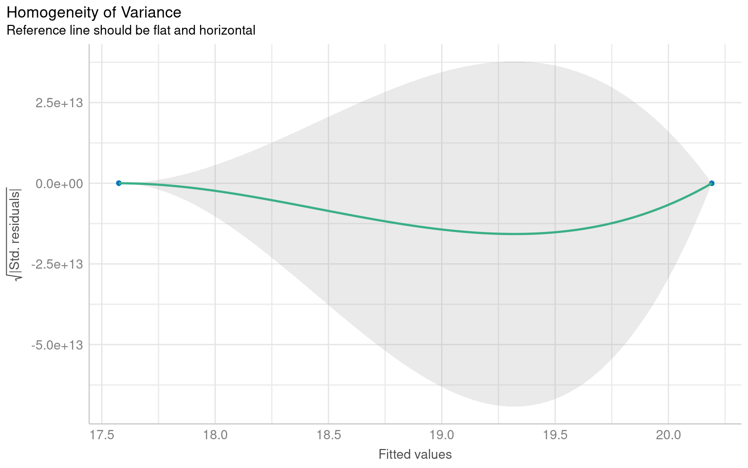
Warning: Non-normality of residuals detected (p < .001).
Warning: Heteroscedasticity (non-constant error variance) detected (p = 0.047).
We don’t have to use performance, base R can visualise these with the plot() function
8.7 Simple write-up
From the Welch t-test (or the linear model), you can write:
“The maize plants that have been cross-pollinated were taller on average than the self-pollinated plants. The mean difference in height was approximately 2.62 inches (95% CI: 0.34 to 4.89), t(df ≈ 28) ≈ 2.35, p ≈ 0.026.”
Tip: Match the df and exact numbers to the specific method you report (Welch vs equal-variance vs robust) as they will be slightly different. Using rstatix::t_test(..., detailed = TRUE) or broom::tidy(..., conf.int = TRUE) ensures you have all values at hand.
NoteEstimating means
One limitation of the table of coefficients output is that it doesn’t provide the mean and standard error of the other treatment level (only the difference between them). If we wish to calculate the “other” mean and SE then we can get R to do this.
8.7.1 Changing the intercept
One way to do this is to change the levels of the type variable as a factor:
# Perform linear regression on darwin data with Self as the intercept
darwin |>
  # Convert 'type' column to a factor
  mutate(type = factor(type)) |>
  # Relevel 'type' column to specify the order of factor levels
  mutate(type = fct_relevel(type, c("Self", "Cross"))) |>
  # Fit linear regression model with 'height' as the response variable and 'type' as the predictor
  lm(height ~ type, data = _) |>
  # Tidy the model summary
broom::tidy()| term | estimate | std.error | statistic | p.value |
|---|---|---|---|---|
| (Intercept) | 17.575000 | 0.7592028 | 23.149282 | 0.0000000 |
| typeCross | 2.616667 | 1.0736749 | 2.437113 | 0.0214145 |
After releveling, the self treatment is now taken as the intercept, and we get the estimate for it’s mean and standard error
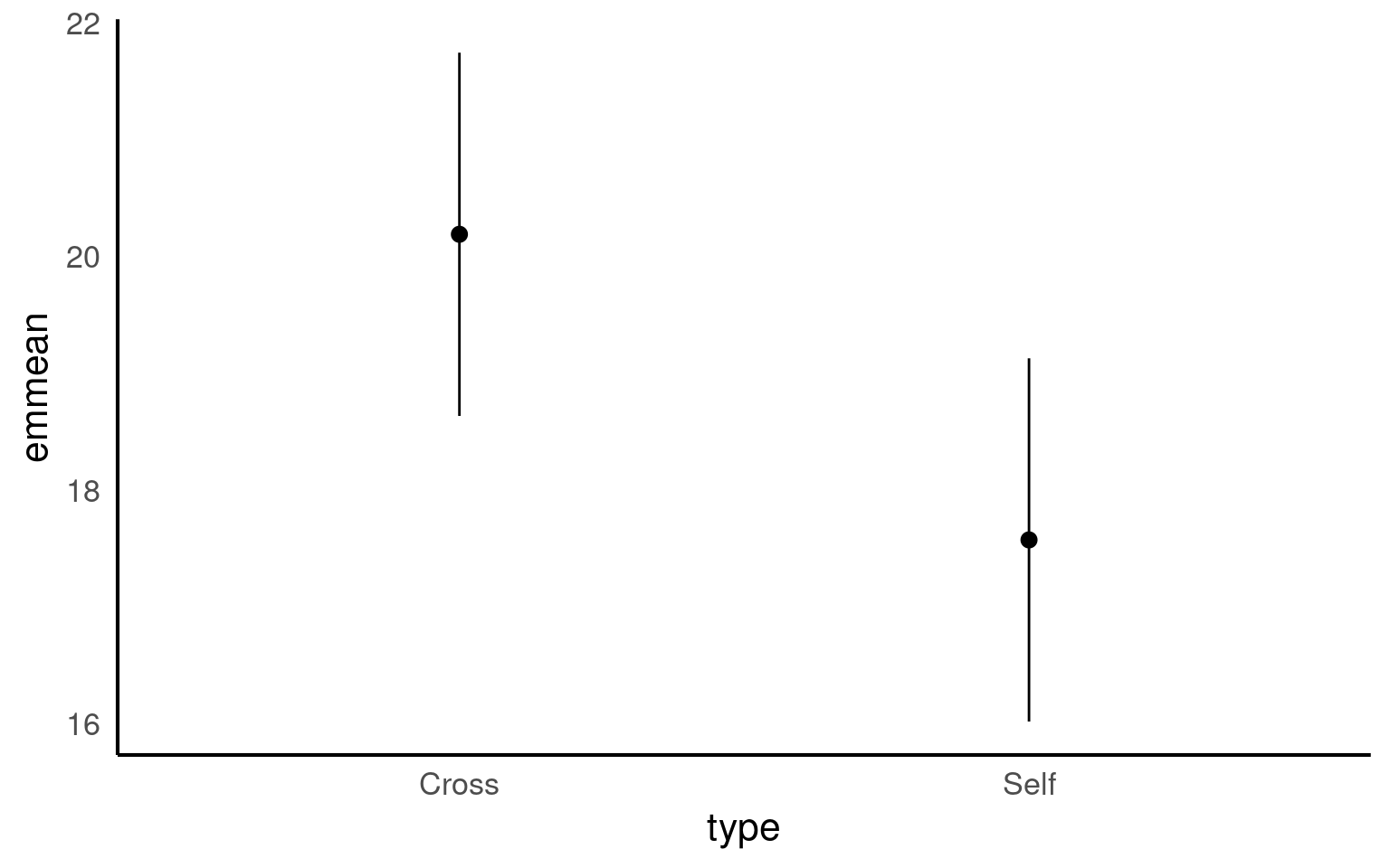
8.7.2 Emmeans
We could also use the package emmeans and its function emmeans() to do a similar thing
 type  emmean    SE df lower.CL upper.CL
 Cross   20.2 0.759 28     18.6     21.7
 Self    17.6 0.759 28     16.0     19.1

Confidence level used: 0.95
The advantage of emmeans is that it provides the mean, standard error and 95% confidence interval estimates of all levels from the model at once (e.g. it relevels the model multiple times behind the scenes).
emmeans also gives us a handy summary to include in data visuals that combine raw data and statistical inferences. These are standard ggplot() outputs so can be customised as much as you want.
Notice that no matter how we calculate the estimated SE (and therefore the 95% CI) of both treatments is the same. This is because as mentioned earlier the variance is a pooled estimate, e.g. variance is not being calculate separately for each group. The only difference you should see in SE across treatments will be if there is a difference in sample size between groups.