| verb | action |
|---|---|
| select() | choose columns by name |
| filter() | select rows based on conditions |
| arrange() | reorder the rows |
| summarise() | reduce raw data to user defined summaries |
| group_by() | group the rows by a specified column |
| mutate() | create a new variable |
3 Data cleaning
In this chapter you will learn how to use tidyverse functions to data clean and wrangle tidy dataTidy data refers to a specific format for organizing datasets that makes data easier to work with for analysis and visualization in R, especially using the tidyverse. The concept was popularized by Hadley Wickham in his paper “Tidy Data” and is an essential principle for effective data manipulation. introduced in Appendix C
3.1 Introduction to dplyr
In this section we will be introduced to some of the most commonly used data wrangling functions, these come from the dplyr package (part of the tidyverse). These are functions you are likely to become very familiar with.
Important
Work in your existing R project
Try running the following functions directly in your consoleThe R console is the interactive interface within the R environment where users can type and execute R code. It is the place where you can directly enter commands, see their output, and interact with the R programming language in real-time. or make a scraps.R scrappy file to mess around in.
3.1.1 Select
If we wanted to create a dataset that only includes certain variables, we can use the dplyr::select() function from the dplyr package.
For example I might wish to create a simplified dataset that only contains species, sex, flipper_length_mm and body_mass_g.
Run the below code to select only those columns
Alternatively you could tell R the columns you don’t want e.g.
Note that select() does not change the original penguins tibble. It spits out the new tibble directly into your console.
If you don’t save this new tibble, it won’t be stored. If you want to keep it, then you must create a new object.
When you run this new code, you will not see anything in your console, but you will see a new object appear in your Environment pane.
3.1.2 Filter
Having previously used dplyr::select() to select certain variables, we will now use dplyr::filter() to select only certain rows or observations. For example only Adelie penguins.
We can do this with the equivalence operator ==
TipOperator confusion
Don’t confuse “=” which assigns a value with “==” which checks if two things are ‘equivalent’. See Section A.5.1 for more.
We can use several different operators to assess the way in which we should filter our data that work the same in tidyverse or base R.
| Operator | Name |
|---|---|
| A < B | less than |
| A <= B | less than or equal to |
| A > B | greater than |
| A >= B | greater than or equal to |
| A == B | equivalence |
| A != B | not equal |
| A %in% B | in |
If you wanted to select all the Penguin species except Adelies, you use ‘not equals’.
This is the same as
You can include multiple expressions within filter() and it will pull out only those rows that evaluate to TRUE for all of your conditions.
For example the below code will pull out only those observations of Adelie penguins where flipper length was measured as greater than 190mm.
3.1.3 Arrange
The function arrange() sorts the rows in the table according to the columns supplied. For example
The data is now arranged in alphabetical order by sex. So all of the observations of female penguins are listed before males.
You can also reverse this with desc()
You can also sort by more than one column, what do you think the code below does?
3.1.4 Mutate
Sometimes we need to create a new variable that doesn’t exist in our dataset. For example we might want to figure out what the flipper length is when factoring in body mass.
To create new variables we use the function mutate().
Note that as before, if you want to save your new column you must save it as an object. Here we are mutating a new column and attaching it to the new_penguins data oject.
3.2 Pipes
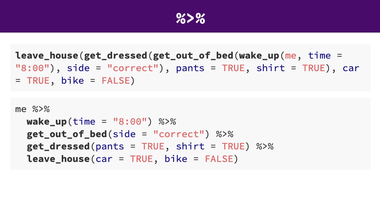
Pipes look like this: |> , a pipeAn operator that allows you to chain multiple functions together in a sequence. allows you to send the output from one function straight into another function. Specifically, they send the result of the function before |> to be the first argument of the function after |>. As usual, it’s easier to show, rather than tell so let’s look at an example.
The reason that this function is called a pipe is because it ‘pipes’ the data through to the next function. When you wrote the code previously, the first argument of each function was the dataset you wanted to work on. When you use pipes it will automatically take the data from the previous line of code so you don’t need to specify it again.
3.2.1 Task
Try and write out as plain English what the |> above is doing? You can read the |> as THEN
Take the penguins data AND THEN Select only the species, sex and flipper length columns AND THEN Filter to keep only those observations labelled as sex equals male AND THEN Arrange the data from HIGHEST to LOWEST flipper lengths.
From R version 4 onwards there is now a “native pipe” |>
This doesn’t require the tidyverse magrittr package and the “old pipe” %>% or any other packages to load and use.
You may be familiar with the magrittr pipe or see it in other tutorials, and website usages. The native pipe works equivalntly in most situations but if you want to read about some of the operational differences, this site does a good job of explaining .
3.3 Clean the Penguin Data
Warning
Re-open your 01_import_penguins_data.R started in Chapter 1 and start to add these commands to your data importing and cleaning script:
3.3.1 Activity 1: Explore data structure
Before working with your data, it’s essential to understand its underlying structure and content. In this section, we’ll use powerful functions like glimpse(), str(), summary(), head(), tail() and the add-on function skimr::skim() to thoroughly examine your dataset. These tools provide insights into data types, variable distributions, and sample records, helping you identify initial issues such as missing values or inconsistent data types. By gaining a clear understanding of your data’s structure, you’ll be better equipped to address any problems and proceed confidently with data cleaning and analysis.
When we run glimpse() we get several lines of output. The number of observations “rows”, the number of variables “columns”. Check this against the csv file you have - they should be the same. In the next lines we see variable names and the type of data.
Rows: 344
Columns: 17
$ studyName             <chr> "PAL0708", "PAL0708", "PAL0708", "PAL0708", "PAL…
$ `Sample Number`       <dbl> 1, 2, 3, 4, 5, 6, 7, 8, 9, 10, 11, 12, 13, 14, 1…
$ Species               <chr> "Adelie Penguin (Pygoscelis adeliae)", "Adelie P…
$ Region                <chr> "Anvers", "Anvers", "Anvers", "Anvers", "Anvers"…
$ Island                <chr> "Torgersen", "Torgersen", "Torgersen", "Torgerse…
$ Stage                 <chr> "Adult, 1 Egg Stage", "Adult, 1 Egg Stage", "Adu…
$ `Individual ID`       <chr> "N1A1", "N1A2", "N2A1", "N2A2", "N3A1", "N3A2", …
$ `Clutch Completion`   <chr> "Yes", "Yes", "Yes", "Yes", "Yes", "Yes", "No", …
$ `Date Egg`            <chr> "11/11/2007", "11/11/2007", "16/11/2007", "16/11…
$ `Culmen Length (mm)`  <dbl> 39.1, 39.5, 40.3, NA, 36.7, 39.3, 38.9, 39.2, 34…
$ `Culmen Depth (mm)`   <dbl> 18.7, 17.4, 18.0, NA, 19.3, 20.6, 17.8, 19.6, 18…
$ `Flipper Length (mm)` <dbl> 181, 186, 195, NA, 193, 190, 181, 195, 193, 190,…
$ `Body Mass (g)`       <dbl> 3750, 3800, 3250, NA, 3450, 3650, 3625, 4675, 34…
$ Sex                   <chr> "MALE", "FEMALE", "FEMALE", NA, "FEMALE", "MALE"…
$ `Delta 15 N (o/oo)`   <dbl> NA, 8.94956, 8.36821, NA, 8.76651, 8.66496, 9.18…
$ `Delta 13 C (o/oo)`   <dbl> NA, -24.69454, -25.33302, NA, -25.32426, -25.298…
$ Comments              <chr> "Not enough blood for isotopes.", NA, NA, "Adult…
We can see a dataset with 345 rows (including the headers) and 17 variables It also provides information on the type of data in each column
<chr>- means character or text data<dbl>- means numerical data
When we run summary() we get similar information, in addition for any numerical values we get summary statistics such as mean, median, min, max, quartile ranges and any missing (NA) values
  studyName         Sample Number      Species             Region
 Length:344         Min.   :  1.00   Length:344         Length:344
 Class :character   1st Qu.: 29.00   Class :character   Class :character
 Mode  :character   Median : 58.00   Mode  :character   Mode  :character
                    Mean   : 63.15
                    3rd Qu.: 95.25
                    Max.   :152.00

    Island             Stage           Individual ID      Clutch Completion
 Length:344         Length:344         Length:344         Length:344
 Class :character   Class :character   Class :character   Class :character
 Mode  :character   Mode  :character   Mode  :character   Mode  :character


   Date Egg         Culmen Length (mm) Culmen Depth (mm) Flipper Length (mm)
 Length:344         Min.   :32.10      Min.   :13.10     Min.   :172.0
 Class :character   1st Qu.:39.23      1st Qu.:15.60     1st Qu.:190.0
 Mode  :character   Median :44.45      Median :17.30     Median :197.0
                    Mean   :43.92      Mean   :17.15     Mean   :200.9
                    3rd Qu.:48.50      3rd Qu.:18.70     3rd Qu.:213.0
                    Max.   :59.60      Max.   :21.50     Max.   :231.0
                    NA's   :2          NA's   :2         NA's   :2
 Body Mass (g)      Sex            Delta 15 N (o/oo) Delta 13 C (o/oo)
 Min.   :2700   Length:344         Min.   : 7.632    Min.   :-27.02
 1st Qu.:3550   Class :character   1st Qu.: 8.300    1st Qu.:-26.32
 Median :4050   Mode  :character   Median : 8.652    Median :-25.83
 Mean   :4202                      Mean   : 8.733    Mean   :-25.69
 3rd Qu.:4750                      3rd Qu.: 9.172    3rd Qu.:-25.06
 Max.   :6300                      Max.   :10.025    Max.   :-23.79
 NA's   :2                         NA's   :14        NA's   :13
   Comments
 Length:344
 Class :character
 Mode  :character
Finally the add-on package skimr provides the function skimr::skim() provides an easy to view set of summaries including column types, completion rate, number of unique variables in each column and similar statistical summaries along with a small histogram for each numeric variable.
| Name | penguins_raw |
| Number of rows | 344 |
| Number of columns | 17 |
| _______________________ | |
| Column type frequency: | |
| character | 10 |
| numeric | 7 |
| ________________________ | |
| Group variables | None |
Variable type: character
| skim_variable | n_missing | complete_rate | min | max | empty | n_unique | whitespace |
|---|---|---|---|---|---|---|---|
| studyName | 0 | 1.00 | 7 | 7 | 0 | 3 | 0 |
| Species | 0 | 1.00 | 33 | 41 | 0 | 3 | 0 |
| Region | 0 | 1.00 | 6 | 6 | 0 | 1 | 0 |
| Island | 0 | 1.00 | 5 | 9 | 0 | 3 | 0 |
| Stage | 0 | 1.00 | 18 | 18 | 0 | 1 | 0 |
| Individual ID | 0 | 1.00 | 4 | 6 | 0 | 190 | 0 |
| Clutch Completion | 0 | 1.00 | 2 | 3 | 0 | 2 | 0 |
| Date Egg | 0 | 1.00 | 10 | 10 | 0 | 50 | 0 |
| Sex | 11 | 0.97 | 4 | 6 | 0 | 2 | 0 |
| Comments | 290 | 0.16 | 18 | 68 | 0 | 10 | 0 |
Variable type: numeric
| skim_variable | n_missing | complete_rate | mean | sd | p0 | p25 | p50 | p75 | p100 | hist |
|---|---|---|---|---|---|---|---|---|---|---|
| Sample Number | 0 | 1.00 | 63.15 | 40.43 | 1.00 | 29.00 | 58.00 | 95.25 | 152.00 | ▇▇▆▅▃ |
| Culmen Length (mm) | 2 | 0.99 | 43.92 | 5.46 | 32.10 | 39.23 | 44.45 | 48.50 | 59.60 | ▃▇▇▆▁ |
| Culmen Depth (mm) | 2 | 0.99 | 17.15 | 1.97 | 13.10 | 15.60 | 17.30 | 18.70 | 21.50 | ▅▅▇▇▂ |
| Flipper Length (mm) | 2 | 0.99 | 200.92 | 14.06 | 172.00 | 190.00 | 197.00 | 213.00 | 231.00 | ▂▇▃▅▂ |
| Body Mass (g) | 2 | 0.99 | 4201.75 | 801.95 | 2700.00 | 3550.00 | 4050.00 | 4750.00 | 6300.00 | ▃▇▆▃▂ |
| Delta 15 N (o/oo) | 14 | 0.96 | 8.73 | 0.55 | 7.63 | 8.30 | 8.65 | 9.17 | 10.03 | ▃▇▆▅▂ |
| Delta 13 C (o/oo) | 13 | 0.96 | -25.69 | 0.79 | -27.02 | -26.32 | -25.83 | -25.06 | -23.79 | ▆▇▅▅▂ |
Q Based on our summary functions are any variables assigned to the wrong data type (should be character when numeric or vice versa)?
Although some columns like date might not be correctly treated as character variables, they are not strictly numeric either, all other columns appear correct
3.3.1.1 Missing Data
Q Based on our summary functions do we have complete data for all variables?
No, they are 2 missing data points for body measurements (culmen, flipper, body mass), 11 missing data points for sex, 13/14 missing data points for blood isotopes (Delta N/C) and 290 missing data points for comments
Sometimes we want to remove rows where values are missing, this will be covered later - for now we just want to be aware of where we do not have complete records.
3.3.2 Activity 2: Clean column names
 [1] "studyName"           "Sample Number"       "Species"
 [4] "Region"              "Island"              "Stage"
 [7] "Individual ID"       "Clutch Completion"   "Date Egg"
[10] "Culmen Length (mm)"  "Culmen Depth (mm)"   "Flipper Length (mm)"
[13] "Body Mass (g)"       "Sex"                 "Delta 15 N (o/oo)"
[16] "Delta 13 C (o/oo)"   "Comments"
When we run colnames() we get the identities of each column in our dataframe
Study name: an identifier for the year in which sets of observations were made
Region: the area in which the observation was recorded
Island: the specific island where the observation was recorded
Stage: Denotes reproductive stage of the penguin
Individual ID: the unique ID of the individual
Clutch completion: if the study nest observed with a full clutch e.g. 2 eggs
Date egg: the date at which the study nest observed with 1 egg
Culmen length: length of the dorsal ridge of the bird’s bill (mm)
Culmen depth: depth of the dorsal ridge of the bird’s bill (mm)
Flipper Length: length of bird’s flipper (mm)
Body Mass: Bird’s mass in (g)
Sex: Denotes the sex of the bird
Delta 15N : the ratio of stable Nitrogen isotopes 15N:14N from blood sample
Delta 13C: the ratio of stable Carbon isotopes 13C:12C from blood sample
3.3.2.1 Clean column names
Often we might want to change the names of our variables. They might be non-intuitive, or too long. Our data has a couple of issues:
Some of the names contain spaces
Some of the names have capitalised letters
Some of the names contain brackets
R is case-sensitive and also doesn’t like spaces or brackets in variable names, because of this we have been forced to use backticks `Sample Number` to prevent errors when using these column names
# CLEAN DATA ----

# clean all variable names to snake_case
# using the clean_names function from the janitor package
# note we are using assign <-
# to overwrite the old version of penguins
# with a version that has updated names
# this changes the data in our R workspace
# but NOT the original csv file

# clean the column names
# assign to new R object
penguins_clean <- janitor::clean_names(penguins_raw)

# quickly check the new variable names
colnames(penguins_clean)
[1] "study_name" "sample_number" "species"
[4] "region" "island" "stage"
[7] "individual_id" "clutch_completion" "date_egg"
[10] "culmen_length_mm" "culmen_depth_mm" "flipper_length_mm"
[13] "body_mass_g" "sex" "delta_15_n_o_oo"
[16] "delta_13_c_o_oo" "comments" 3.3.2.2 Rename columns (manually)
The clean_names function quickly converts all variable names into snake caseSnake case is a naming convention in computing that uses underscores to replace spaces between words, and writes words in lowercase. It’s commonly used for variable names, filenames, and database table and column names.. The N and C blood isotope ratio names are still quite long though, so let’s clean those with dplyr::rename() where “new_name” = “old_name”.
3.3.2.3 Rename text values manually
Sometimes we may want to rename the values in our variables in order to make a shorthand that is easier to follow. This is changing the values in our columns, not the column names.
# use mutate and case_when
# for a statement that conditionally changes
# the names of the values in a variable
penguins <- penguins_clean |>
  mutate(species = case_when(
  species == "Adelie Penguin (Pygoscelis adeliae)" ~ "Adelie",
  species == "Gentoo penguin (Pygoscelis papua)" ~ "Gentoo",
  species == "Chinstrap penguin (Pygoscelis antarctica)" ~ "Chinstrap",
  .default = as.character(species)
  )
  )
Warning
Notice from here on out I am assigning the output of my code to the R object penguins, this means any new code “overwrites” the old penguins dataframe. This is because I ran out of new names I could think of, its also because my Environment is filling up with lots of data frame variants.
Be aware that when you run code in this way, it can cause errors if you try to run the same code twice e.g. in the example above once you have changed MALE to Male, running the code again could cause errors as MALE is no longer present!
If you make any mistakes running code in this way, re-start your R session and run the code from the start to where you went wrong.
Have you checked that the above code block worked? Inspect your new tibble and check the variables have been renamed as you wanted.
3.3.2.4 Rename text values with stringr
Datasets often contain words, and we call these words “(character) strings”.
Often these aren’t quite how we want them to be, but we can manipulate these as much as we like. Functions in the package stringr, are fantastic. And the number of different types of manipulations are endless!
Below we repeat the outcomes above, but with string matching:
Alternatively we could decide we want simpler species names but that we would like to keep the latin name information, but in a separate column. To do this we are using regex. Regular expressions are a concise and flexible tool for describing patterns in strings
| study_name | sample_number | species | full_latin_name | region | island | stage | individual_id | clutch_completion | date_egg | culmen_length_mm | culmen_depth_mm | flipper_length_mm | body_mass_g | sex | delta_15n | delta_13c | comments |
|---|---|---|---|---|---|---|---|---|---|---|---|---|---|---|---|---|---|
| PAL0708 | 1 | Adelie Penguin | (Pygoscelis adeliae) | Anvers | Torgersen | Adult, 1 Egg Stage | N1A1 | Yes | 11/11/2007 | 39.1 | 18.7 | 181 | 3750 | MALE | NA | NA | Not enough blood for isotopes. |
| PAL0708 | 2 | Adelie Penguin | (Pygoscelis adeliae) | Anvers | Torgersen | Adult, 1 Egg Stage | N1A2 | Yes | 11/11/2007 | 39.5 | 17.4 | 186 | 3800 | FEMALE | 8.94956 | -24.69454 | NA |
| PAL0708 | 3 | Adelie Penguin | (Pygoscelis adeliae) | Anvers | Torgersen | Adult, 1 Egg Stage | N2A1 | Yes | 16/11/2007 | 40.3 | 18.0 | 195 | 3250 | FEMALE | 8.36821 | -25.33302 | NA |
| PAL0708 | 4 | Adelie Penguin | (Pygoscelis adeliae) | Anvers | Torgersen | Adult, 1 Egg Stage | N2A2 | Yes | 16/11/2007 | NA | NA | NA | NA | NA | NA | NA | Adult not sampled. |
| PAL0708 | 5 | Adelie Penguin | (Pygoscelis adeliae) | Anvers | Torgersen | Adult, 1 Egg Stage | N3A1 | Yes | 16/11/2007 | 36.7 | 19.3 | 193 | 3450 | FEMALE | 8.76651 | -25.32426 | NA |
| PAL0708 | 6 | Adelie Penguin | (Pygoscelis adeliae) | Anvers | Torgersen | Adult, 1 Egg Stage | N3A2 | Yes | 16/11/2007 | 39.3 | 20.6 | 190 | 3650 | MALE | 8.66496 | -25.29805 | NA |
3.3.3 Activity 2: Checking for duplications
It is very easy when inputting data to make mistakes, copy something in twice for example, or if someone did a lot of copy-pasting to assemble a spreadsheet (yikes!). We can check this pretty quickly
[1] 0Great!
If I did have duplications I could investigate further and extract these exact rows:
A tibble:0 × 17
0 rows | 1-8 of 17 columns| study_name | sample_number | species | region | island | stage | individual_id | clutch_completion | date_egg | culmen_length_mm | culmen_depth_mm | flipper_length_mm | body_mass_g | sex | delta_15n | delta_13c | comments |
|---|---|---|---|---|---|---|---|---|---|---|---|---|---|---|---|---|
| PAL0708 | 1 | Adelie | Anvers | Torgersen | Adult, 1 Egg Stage | N1A1 | Yes | 11/11/2007 | 39.1 | 18.7 | 181 | 3750 | Male | NA | NA | Not enough blood for isotopes. |
| PAL0708 | 2 | Adelie | Anvers | Torgersen | Adult, 1 Egg Stage | N1A2 | Yes | 11/11/2007 | 39.5 | 17.4 | 186 | 3800 | Female | 8.94956 | -24.69454 | NA |
| PAL0708 | 3 | Adelie | Anvers | Torgersen | Adult, 1 Egg Stage | N2A1 | Yes | 16/11/2007 | 40.3 | 18.0 | 195 | 3250 | Female | 8.36821 | -25.33302 | NA |
| PAL0708 | 4 | Adelie | Anvers | Torgersen | Adult, 1 Egg Stage | N2A2 | Yes | 16/11/2007 | NA | NA | NA | NA | NA | NA | NA | Adult not sampled. |
| PAL0708 | 5 | Adelie | Anvers | Torgersen | Adult, 1 Egg Stage | N3A1 | Yes | 16/11/2007 | 36.7 | 19.3 | 193 | 3450 | Female | 8.76651 | -25.32426 | NA |
| PAL0708 | 6 | Adelie | Anvers | Torgersen | Adult, 1 Egg Stage | N3A2 | Yes | 16/11/2007 | 39.3 | 20.6 | 190 | 3650 | Male | 8.66496 | -25.29805 | NA |
3.3.4 Activity 3: Checking for typos
We can also look for typos by asking R to produce all of the distinct values in a variable. This is more useful for categorical data, where we expect there to be only a few distinct categories
Here if someone had mistyped e.g. ‘FMALE’ it would be obvious. We could do the same thing (and probably should have before we changed the names) for species.
We can also trim leading or trailing empty spaces with stringr::str_trim. These are often problematic and difficult to spot e.g.
| label |
|---|
| penguin |
| penguin |
| penguin |
We can easily imagine a scenario where data is manually input, and trailing or leading spaces are left in. These are difficult to spot by eye - but problematic because as far as R is concerned these are different values. We can use the function distinct to return the names of all the different levels it can find in this dataframe.
If we pipe the data throught the str_trim function to remove any gaps, then pipe this on to distinct again - by removing the whitespace, R now recognises just one level to this data.
3.4 Working with dates
Working with dates can be tricky, treating date as strictly numeric is problematic, it won’t account for number of days in months or number of months in a year.
Additionally there’s a lot of different ways to write the same date:
13-10-2019
10-13-2019
13-10-19
13th Oct 2019
2019-10-13
This variability makes it difficult to tell our software how to read the information, luckily we can use the functions in the lubridate package.
If you get a warning that some dates could not be parsed, then you might find the date has been inconsistently entered into the dataset.
Pay attention to warning and error messages
Depending on how we interpret the date ordering in a file, we can use ymd(), ydm(), mdy(), dmy()
-
Question What is the appropriate function from the above to use on the
date_eggvariable?
Here we use the mutate function from dplyr to create a new variable called date_egg_proper based on the output of converting the characters in date_egg to date format. The original variable is left intact, if we had specified the “new” variable was also called date_egg then it would have overwritten the original variable.
Once we have established our date data, we are able to perform calculations or extract information. Such as the date range across which our data was collected.
3.4.1 Calculations with dates
ImportantCheck your outputs
Check that this code is producing sensible outputs - it will not work if you have skipped making the necessary column for dates date_egg
We can also extract and make new columns from our date column - such as a simple column of the year when each observation was made:
3.5 Factors
In R, factors are a class of data that allow for ordered categories with a fixed set of acceptable values.
Typically, you would convert a column from character to a factor if you want to set an intrinsic order to the values (“levels”) so they can be displayed non-alphabetically in plots and tables, or for use in linear model analyses (more on this later).
ImportantWhen to apply factors
Factors provide order to categorical data - you should not assign factors to numeric data - the exception might be if you wanted to bin data into groups (see below)
Working with factors is easy with the forcats package:
Using dplyr::across() - we can apply functions to columns based on selected criteria - here within mutate we are changing each column in the .cols argument and applying the function forcats::as_factor()
Rows: 344
Columns: 5
$ species <fct> Adelie, Adelie, Adelie, Adelie, Adelie, Adelie, Adelie, Adelie…
$ region <fct> Anvers, Anvers, Anvers, Anvers, Anvers, Anvers, Anvers, Anvers…
$ island <fct> Torgersen, Torgersen, Torgersen, Torgersen, Torgersen, Torgers…
$ stage <fct> "Adult, 1 Egg Stage", "Adult, 1 Egg Stage", "Adult, 1 Egg Stag…
$ sex <fct> Male, Female, Female, NA, Female, Male, Female, Male, NA, NA, …
Important
Unless we assign the output of this code to an R object it will just print into the console, in the above I am demonstrating how to change variables to factors but we aren’t “saving” this change.
3.5.1 Setting factor levels
If we want to specify the correct order for a factor we can use forcats::fct_relevel.
In this example we have decided to categorise our penguins into groups - “smol”, “mid” and “chonk” based on mass (g), first we need to create a new column (mass range).
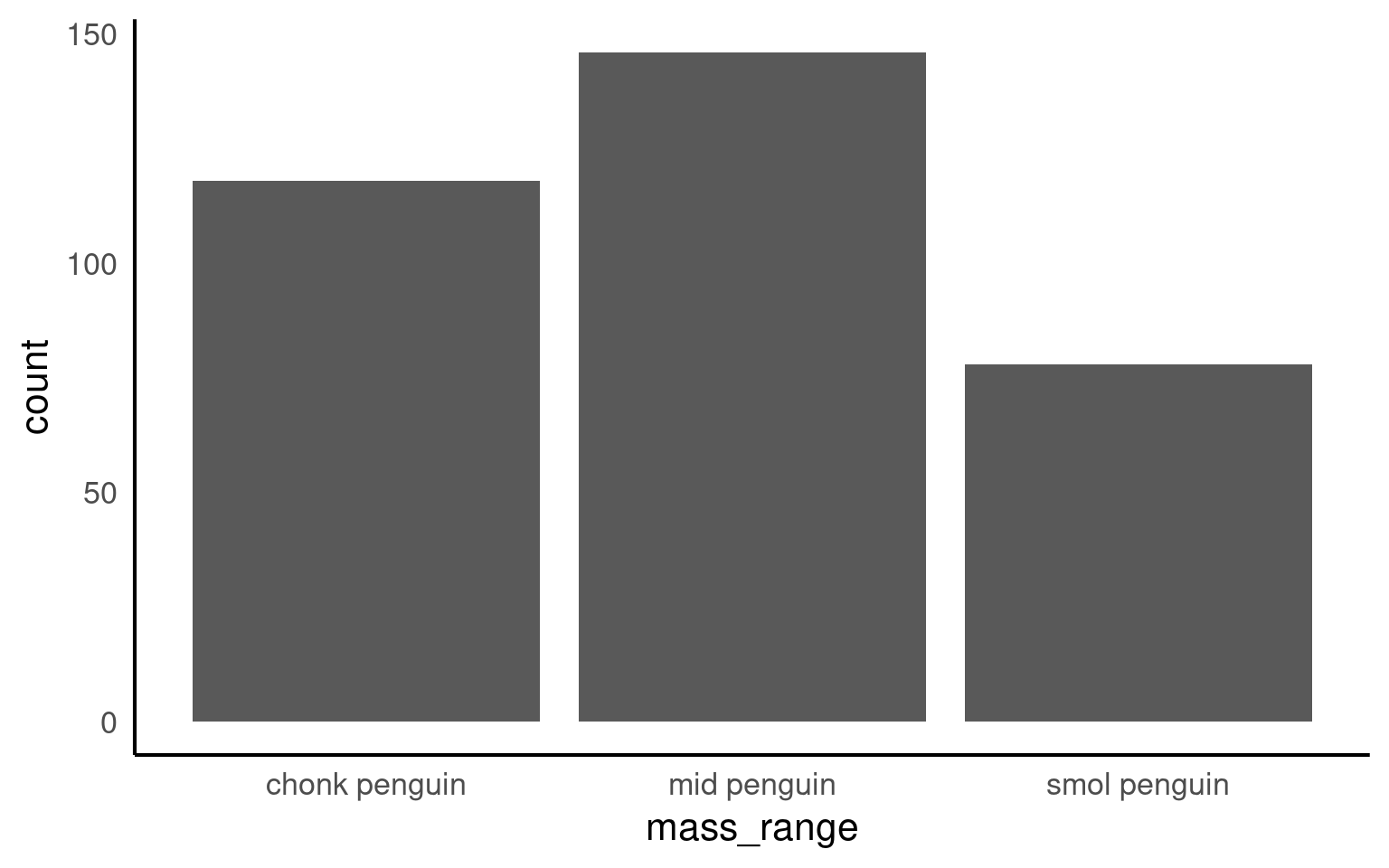
If we make a barplot, the order of the values on the x axis will typically be in alphabetical order for any character data
To convert a character or numeric column to class factor, you can use any function from the forcats package. They will convert to class factor and then also perform or allow certain ordering of the levels - for example using forcats::fct_relevel() lets you manually specify the level order.
The function as_factor() simply converts the class without any further capabilities.
Below we use mutate() and as_factor() to convert the column flipper_range from class character to class factor.
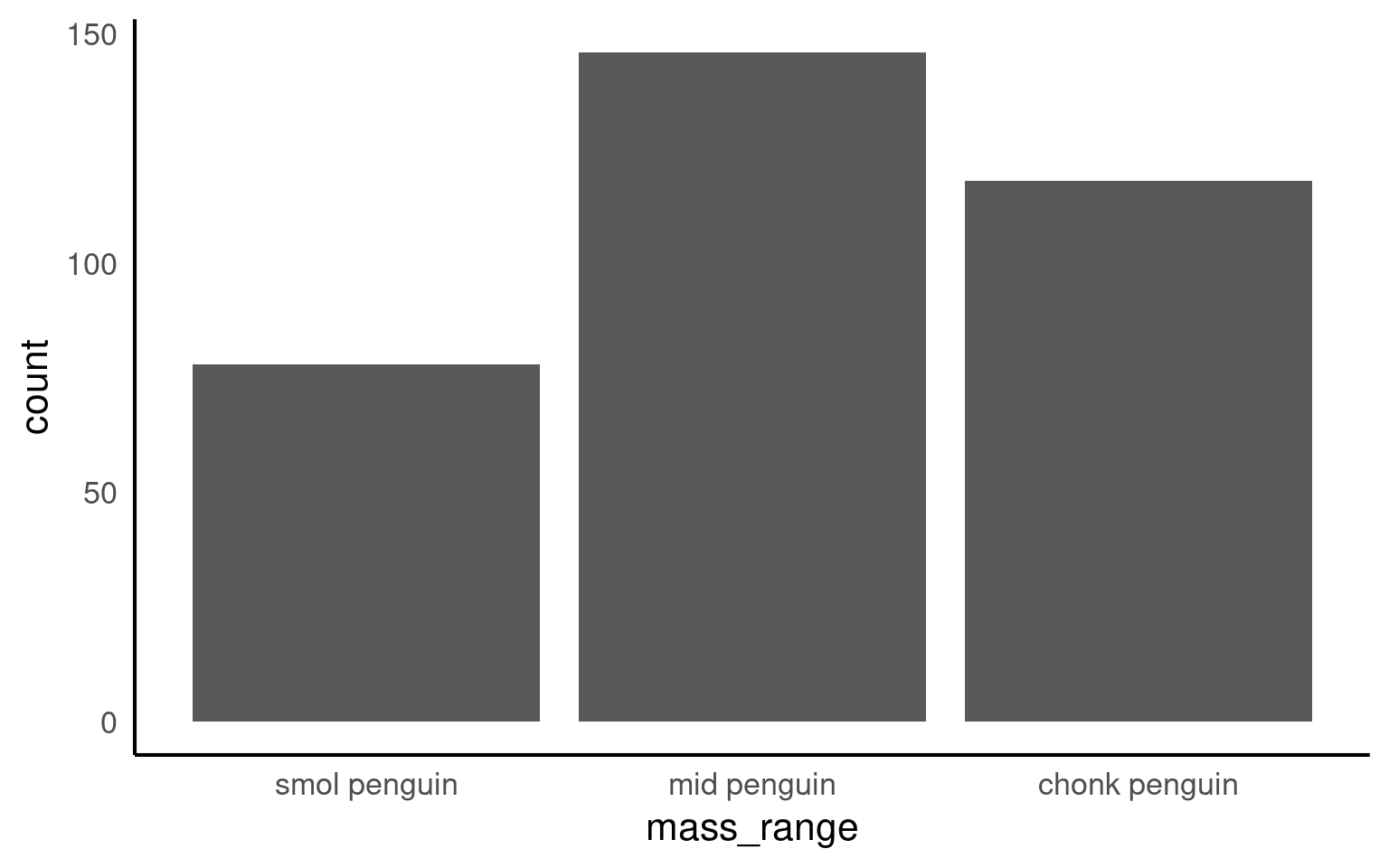
[1] "smol penguin" "mid penguin" "chonk penguin"Now when we call a plot, we can see that the x axis categories match the intrinsic order we have specified with our factor levels.
Factors will also be important when we build linear models a bit later. The reference or intercept for a categorical predictor variable when it is read as a <chr> is set by R as the first one when ordered alphabetically. This may not always be the most appropriate choice, and by changing this to an ordered <fct> we can manually set the intercept.
3.6 Summary
In this chapter we have successfully imported and checked our data for typos and small errors, we have also been introduce to some of the key functions in the dplyr package for data wrangling. Now that we have confidence in the format and integrity of our data, next time we will start to make insights and understand patterns.
3.6.1 Save scripts & data
- Having produced a handy cleaned penguins dataset, we could choose to save it - this will reduce computation in the future as we have a tidied dataset we can work with directly. To do this we can use the
readr::write_csv()function:
- Make sure you have saved your script 💾 and given it the filename
01_import_penguins_data.Rit should be saved in your scripts folder.
ImportantOrganised scripts
Don’t just check the content of your script is the same as the example below. Check that layouts are clear and comments have been included.
#___________________________----
# SET UP ----
# An analysis of the bill dimensions of male and female
# Adelie, Gentoo and Chinstrap penguins
# Data first published in Gorman, KB, TD Williams, and WR Fraser.
# 2014.
# “Ecological Sexual Dimorphism and Environmental Variability
# Within a Community of Antarctic Penguins (Genus Pygoscelis).”
# PLos One 9 (3): e90081.
# https://doi.org/10.1371/journal.pone.0090081.
#__________________________----
# PACKAGES ----
library(tidyverse) # tidy data packages
library(here) # organised file paths
library(janitor) # cleans variable names
#__________________________----
# IMPORT DATA ----
penguins_raw <- read_csv(here("data", "raw", "penguins_raw.csv"))
# check the data has loaded, prints first 10 rows of dataframe
penguins_raw
#__________________________----
# CLEAN DATA ----
# clean all variable names to snake_case
# using the clean_names function from the janitor package
# note we are using assign <-
# to overwrite the old version of penguins
# with a version that has updated names
# this changes the data in our R workspace
# but NOT the original csv file
# clean the column names
# assign to new R object
penguins_clean <- janitor::clean_names(penguins_raw)
# quickly check the new variable names
colnames(penguins_clean)
# shorten the variable names for N and C isotope blood samples
penguins_clean <- rename(penguins_clean,
"delta_15n" = "delta_15_n_o_oo", # use rename from the dplyr package
"delta_13c" = "delta_13_c_o_oo"
)
# use mutate and case_when for a statement that conditionally changes the names of the values in a variable
penguins <- penguins_clean |>
mutate(species = case_when(
species == "Adelie Penguin (Pygoscelis adeliae)" ~ "Adelie",
species == "Gentoo penguin (Pygoscelis papua)" ~ "Gentoo",
species == "Chinstrap penguin (Pygoscelis antarctica)" ~ "Chinstrap"
))
# use mutate and if_else
# for a statement that conditionally changes
# the names of the values in a variable
penguins <- penguins |>
mutate(sex = if_else(
sex == "MALE", "Male", "Female"
))
# use lubridate to format date and extract the year
penguins <- penguins |>
mutate(date_egg = lubridate::dmy(date_egg))
penguins <- penguins |>
  mutate(year = lubridate::year(date_egg))
# Set body mass ranges
penguins <- penguins |>
mutate(mass_range = case_when(
body_mass_g <= 3500 ~ "smol penguin",
body_mass_g > 3500 & body_mass_g < 4500 ~ "mid penguin",
body_mass_g >= 4500 ~ "chonk penguin",
.default = NA
))
# Assign these to an ordered factor
penguins <- penguins |>
mutate(mass_range = fct_relevel(
mass_range,
"smol penguin",
"mid penguin",
"chonk penguin"
))
# Write our cleaned dataframe to the processed data subfolder
write_csv(
penguins,
"data/processed/penguins_clean.csv"
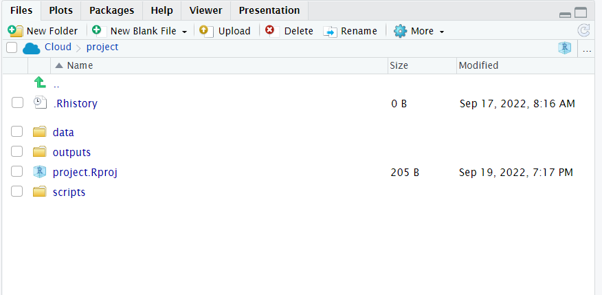
)- Does your workspace look like the below?
- Does your script run from a blank slateR projects are set not to store their .Rhistory file, which means everything required to recreate your analysis is contained in your scripts. without errors as described in Appendix B
ImportantCheck your script runs without error
3.6.2 Checklist for data checking
-
Is each column assigned to the correct data type?
- Are dates formatted correctly?
- Are factors set where needed, are the levels in the correct order?
Are variables consistently named (e.g. using a naming convention such as snake_case)?
Are text values in an appropriate format?
Do we have any data duplication?
Do we have any missing data?
Are there any typos or mistakes in character strings?
3.7 Activity: Test yourself
Question 1. In order to subset a data by rows I should use the function
Question 2. In order to subset a data by columns I should use the function
Question 3. In order to make a new column I should use the function
Question 4. Which operator should I use to send the output from line of code into the next line?
Question 5. What will be the outcome of the following line of code?
Unless the output of a series of functions is “assigned” to an object using <- it will not be saved, the results will be immediately printed. This code would have to be modified to the below in order to create a new filtered object penguins_filtered
Question 6. What is the main point of a data “pipe”?
Question 7. The naming convention outputted by the function `janitor::clean_names() is
Question 8. Which package provides useful functions for manipulating character strings?
Question 9. Which package provides useful functions for manipulating dates?
Question 10. If we do not specify a character variable as a factor, then ordering will default to what?
3.8 Glossary
| term | definition |
|---|---|
| blank slate | R projects are set not to store their .Rhistory file, which means everything required to recreate your analysis is contained in your scripts. |
| console | The R console is the interactive interface within the R environment where users can type and execute R code. It is the place where you can directly enter commands, see their output, and interact with the R programming language in real-time. |
| pipe | An operator that allows you to chain multiple functions together in a sequence. |
| snake case | Snake case is a naming convention in computing that uses underscores to replace spaces between words, and writes words in lowercase. It's commonly used for variable names, filenames, and database table and column names. |
| tidy data | Tidy data refers to a specific format for organizing datasets that makes data easier to work with for analysis and visualization in R, especially using the tidyverse. The concept was popularized by Hadley Wickham in his paper "Tidy Data" and is an essential principle for effective data manipulation. |