4 Worked Example 2 - Nested design
This experiment involved a simple one-way anova with 3 treatments given to 6 rats, the researchers the measured glycogen levels in their liver. The analysis was complicated by the fact that three preparations were taken from the liver of each rat, and two readings of glycogen content were taken from each preparation. This generated 6 pseudoreplicates per rat to give a total of 36 readings in all.
Clearly, it would be a mistake to analyse these data as if they were a straightforward one-way anova, because that would give us 33 degrees of freedom for error. In fact, since there are only two rats in each treatment, we have only one degree of freedom per treatment, giving a total of 3 d.f. for error.
The variance is likely to be different at each level of this nested analysis because:
the readings differ because of variation in the glycogen detection method within each liver sample (measurement error); the pieces of liver may differ because of heterogeneity in the distribution of glycogen within the liver of a single rat; the rats will differ from one another in their glycogen levels because of sex, age, size, genotype, etc.; rats allocated different experimental treatments may differ as a result of the fixed effects of treatment. If all we want to test is whether the experimental treatments have affected the glycogen levels, then we are not interested in liver bits within rat’s livers, or in preparations within liver bits. We could combine all the pseudoreplicates together, and analyse the 6 averages. This would have the virtue of showing what a tiny experiment this really was. This latter approach also ignores the nested sources of uncertainties. Instead we will use a linear mixed model.
rats <- readRDS("rats.rds") Glycogen Rat Treatment Liver
1 131 1 1 1
2 130 1 1 1
3 131 1 1 2
4 125 1 1 2
5 136 1 1 3
6 142 1 1 3
7 150 2 1 1
8 148 2 1 1
9 140 2 1 2
10 143 2 1 2
11 160 2 1 3
12 150 2 1 3
13 157 3 2 1
14 145 3 2 1
15 154 3 2 2
16 142 3 2 2
17 147 3 2 3
18 153 3 2 3
19 151 4 2 1
20 155 4 2 1
21 147 4 2 2
22 147 4 2 2
23 162 4 2 3
24 152 4 2 3
25 134 5 3 1
26 125 5 3 1
27 138 5 3 2
28 138 5 3 2
29 135 5 3 3
30 136 5 3 3
31 138 6 3 1
32 140 6 3 1
33 139 6 3 2
34 138 6 3 2
35 134 6 3 3
36 127 6 3 3
rats_lmer.1 <- lmer(Glycogen ~ Treatment + (1 | Rat) + (1 | Liver), data = rats)
summary(rats_lmer.1)
## Linear mixed model fit by REML. t-tests use Satterthwaite's method [
## lmerModLmerTest]
## Formula: Glycogen ~ Treatment + (1 | Rat) + (1 | Liver)
## Data: rats
##
## REML criterion at convergence: 221.9
##
## Scaled residuals:
## Min 1Q Median 3Q Max
## -1.79334 -0.66536 0.01792 0.59281 2.05206
##
## Random effects:
## Groups Name Variance Std.Dev.
## Rat (Intercept) 39.187 6.260
## Liver (Intercept) 2.168 1.472
## Residual 30.766 5.547
## Number of obs: 36, groups: Rat, 6; Liver, 3
##
## Fixed effects:
## Estimate Std. Error df t value Pr(>|t|)
## (Intercept) 140.500 4.783 3.174 29.373 5.65e-05 ***
## Treatment2 10.500 6.657 3.000 1.577 0.213
## Treatment3 -5.333 6.657 3.000 -0.801 0.482
## ---
## Signif. codes: 0 '***' 0.001 '**' 0.01 '*' 0.05 '.' 0.1 ' ' 1
##
## Correlation of Fixed Effects:
## (Intr) Trtmn2
## Treatment2 -0.696
## Treatment3 -0.696 0.500Q. Why is this model above wrong
It is wrong because this would add two random effect terms, one for rat 1 and one for rat 2. In fact there are 6 rats altogether. The way that the data have been coded allows for these kinds of mistakes to happen. The same is true for Liver, which is coded as a 1, 2 or 3. This means that we could write this thinking that we are including the correct random effects for Rat and Liver. In fact, this assumes that the data come from a crossed design, in which there are 2 rats and 3 parts of the liver, and that Liver = 1 corresponds to the same type of measurement in rats 1 and 2 and so on. Sometimes this is appropriate, but not here!
The nature of the way that many data sets are coded makes these kinds of mistakes very easy to make!
A better design is the one below:
## Linear mixed model fit by REML. t-tests use Satterthwaite's method [
## lmerModLmerTest]
## Formula: Glycogen ~ Treatment + (1 | Rat/Liver)
##    Data: rats
##
## REML criterion at convergence: 219.6
##
## Scaled residuals:
##      Min       1Q   Median       3Q      Max
## -1.48212 -0.47263  0.03062  0.42934  1.82935
##
## Random effects:
##  Groups    Name        Variance Std.Dev.
##  Liver:Rat (Intercept) 14.17    3.764
##  Rat       (Intercept) 36.06    6.005
##  Residual              21.17    4.601
## Number of obs: 36, groups:  Liver:Rat, 18; Rat, 6
##
## Fixed effects:
##             Estimate Std. Error      df t value Pr(>|t|)
## (Intercept)  140.500      4.707   3.000  29.848 8.26e-05 ***
## Treatment2    10.500      6.657   3.000   1.577    0.213
## Treatment3    -5.333      6.657   3.000  -0.801    0.482
## ---
## Signif. codes:  0 '***' 0.001 '**' 0.01 '*' 0.05 '.' 0.1 ' ' 1
##
## Correlation of Fixed Effects:
##            (Intr) Trtmn2
## Treatment2 -0.707
## Treatment3 -0.707  0.500
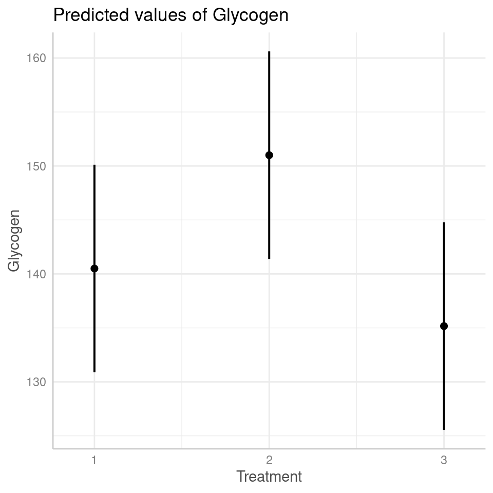
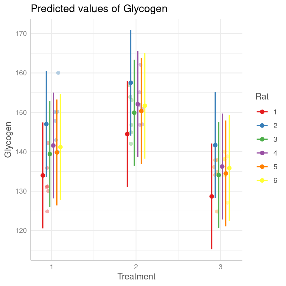
And we can see the effects in the figures below:

