2 Worked Example 1 - Dolphins

2.1 How do I decide if it is a fixed or random effect?

One of the most common questions in mixed-effects modelling is how to decide if an effect should be considered as fixed or random. This can be quite a complicated question, as we have touched upon briefly before the definition of a random effect is not universal. It is a considered process that can include the hypothesis or question you are asking.

1 ) Are you directly interested in the effect in question. If the answer is yes it should be a fixed effect.

2 ) Is the variable continuous? If the answer is yes it should be a fixed effect.

3 ) Does the variable have less than five levels? If ther answer is yes it should be a fixed effect.

2.2 Dolphins

This dataset was collected to measure resting lung function in 32 bottlenose dolphins. The main dependent variable was the tidal volume (\(V_T\)) measured in litres, as an index of lung capacity.

dolphins <- read_csv("files/dolphins.csv") 

dolphins$direction <- factor(dolphins$direction)

dolphins <- drop_na(dolphins)

Here we are interested in the relationship between (\(V_T\)) and body mass (kg), we have measurements which are taken on the breath in and the breath out, and each dolphin has been observed between one and four times.

We need to determine our fixed effects, random effects and model structure:

1. Body Mass Random Effect Fixed Effect

2. Direction Random Effect Fixed Effect

3. Animal 1) Body Mass Random Effect Fixed Effect

4. With the basic structure y ~ x + z + (1|group) what do you think this model should be?:

1. We are clearly interested in the effect of body mass on (\(V_T\)) so this is a fixed effect.

2. We may think that the relationship with (\(V_T\)) and body mass may be different on the in and out breath. We may not be directly interested in this, but it has fewer than fivel levels so this is a fixed effect. (outbreath coded as 1, inbreath coded as 2).

3. Individual dolphins - if we averaged across measurements for each dolphin, our measurement precision would be different for each animal. If we include each data point, we would be double-counting some animals and our observations would not be independent. To account for the multiple observations we should treat animal as a random effect.

dolphmod <- lmer(vt ~ bodymass + direction + (1|animal), data=dolphins)

With our basic linear model in place - we should carry out model fit checks with DHARMa or performance::check_model(), but assuming this is a good fit we can look at interpretation:

summary(dolphmod)

## Linear mixed model fit by REML. t-tests use Satterthwaite's method [
## lmerModLmerTest]
## Formula: vt ~ bodymass + direction + (1 | animal)
##    Data: dolphins
## 
## REML criterion at convergence: 387.4
## 
## Scaled residuals: 
##      Min       1Q   Median       3Q      Max 
## -2.30795 -0.51983  0.04156  0.62404  2.26396 
## 
## Random effects:
##  Groups   Name        Variance Std.Dev.
##  animal   (Intercept) 1.039    1.019   
##  Residual             1.158    1.076   
## Number of obs: 112, groups:  animal, 31
## 
## Fixed effects:
##              Estimate Std. Error        df t value Pr(>|t|)    
## (Intercept)  2.226398   0.627115 28.758081   3.550  0.00135 ** 
## bodymass     0.016782   0.003259 26.720390   5.150  2.1e-05 ***
## direction2   1.114821   0.203389 77.414421   5.481  5.1e-07 ***
## ---
## Signif. codes:  0 '***' 0.001 '**' 0.01 '*' 0.05 '.' 0.1 ' ' 1
## 
## Correlation of Fixed Effects:
##            (Intr) bdymss
## bodymass   -0.927       
## direction2 -0.162  0.000

dolphins.1 <- dolphins %>% 
    mutate(fit.m = predict(dolphmod, re.form = NA),
           fit.c = predict(dolphmod, re.form = NULL))

dolphins.1 %>%
  ggplot(aes(x = bodymass, y = vt, group = direction)) +
  geom_point(pch = 16, aes(colour = direction)) +
  geom_line(aes(y = fit.m, 
                linetype = direction), 
            linewidth = 1)  +
  labs(x = "Body Mass", 
       y = "VT") 

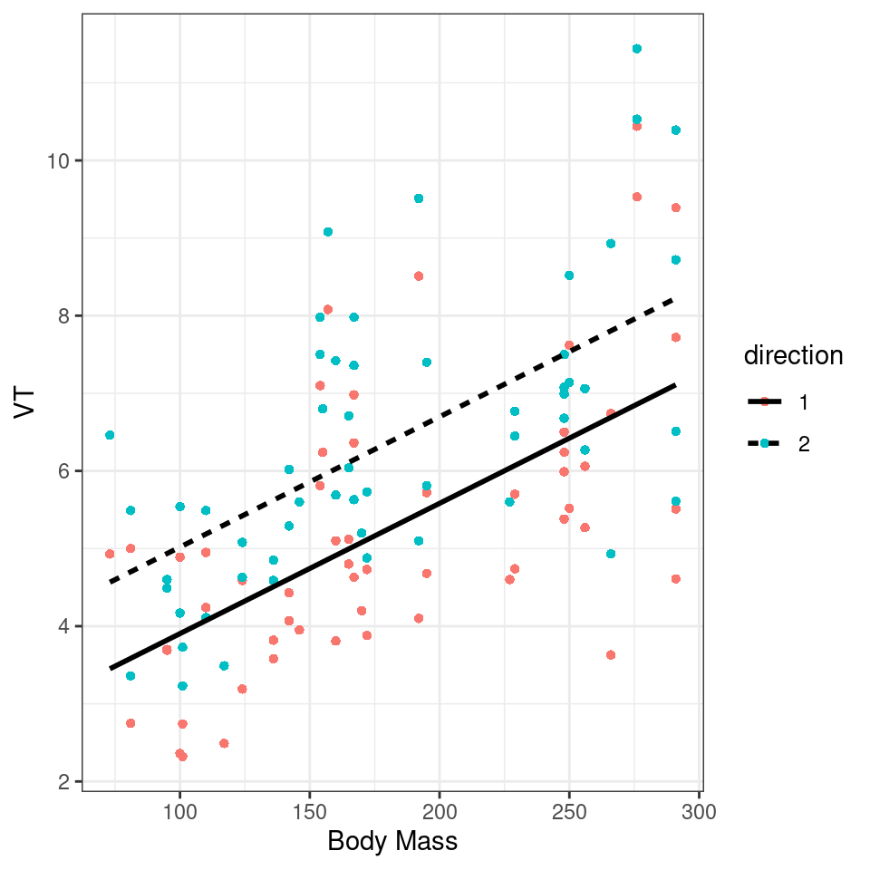
Figure 2.1: Scatter plot of VT as a function of body mass for dolphins. Different directions of breath are represented by different colors. The solid lines indicate the marginal fitted values from our model.

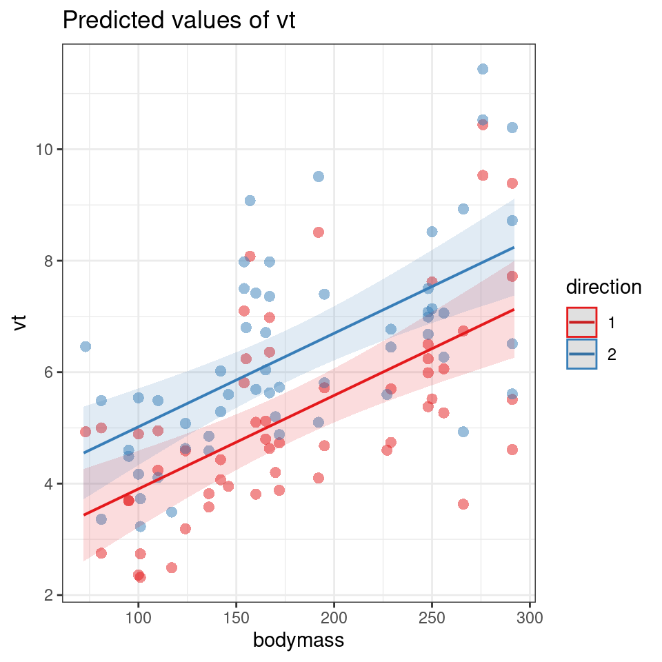
plot_model(dolphmod,type="pred",
           terms=c("bodymass", "direction"),
           pred.type="fe",
           show.data = T)

We fitted a linear mixed model (estimated using REML and nloptwrap optimizer) to predict (\(V_T\)) with bodymass(kg) and direction (in/out breath). 95% Confidence Intervals (CIs) and p-values were computed using a Wald t-distribution approximation. We included a random intercept effect of animal to account for repeated measurements (of between 1 to 4 observations) across a total of 32 bottlenosed dolphins.

We found that for every 1kg increase in bodymass, (\(V_T\)) increased by 0.02 litres (95% CI [0.01 - 0.02]), . The inbreath had on average a higher volume than the outbreath (1.11 litre difference [0.71 - 1.52]..

Q. This is not a perfect write-up, what else could we consider including?