7 Reporting Mixed Model Results

Once you get your model, you have to present it in an accurate, clear and attractive form.

The summary() function provides us with some useful numbers such as the amount of variance left over after fitting our fixed effects that can be assigned to each of our random effects. It also provides information on how correlated our random effects are, which may be of interest in understanding the structure of our data as well.

We can use it to check that the modelled random effect structure matches our data.

It includes the coefficient estimates, t-statistics and p-values of our fixed effects

bio.lmer2 <- lmer(Shoot2 ~ Diversity2 + (Diversity2|Site) + (1 | Site:Mix) + (1|Mix) + (1 | Block), data = biodepth)

summary(bio.lmer2)

## Linear mixed model fit by REML. t-tests use Satterthwaite's method [
## lmerModLmerTest]
## Formula: Shoot2 ~ Diversity2 + (Diversity2 | Site) + (1 | Site:Mix) +  
##     (1 | Mix) + (1 | Block)
##    Data: biodepth
## 
## REML criterion at convergence: 6045.1
## 
## Scaled residuals: 
##     Min      1Q  Median      3Q     Max 
## -2.4340 -0.4698 -0.0866  0.3430  3.5258 
## 
## Random effects:
##  Groups   Name        Variance Std.Dev. Corr
##  Site:Mix (Intercept) 20077.6  141.70       
##  Mix      (Intercept) 15857.6  125.93       
##  Block    (Intercept)   520.6   22.82       
##  Site     (Intercept) 17106.8  130.79       
##           Diversity2   1363.2   36.92   1.00
##  Residual             16747.3  129.41       
## Number of obs: 451, groups:  Site:Mix, 227; Mix, 192; Block, 15; Site, 8
## 
## Fixed effects:
##             Estimate Std. Error      df t value Pr(>|t|)    
## (Intercept)  346.322     52.004   7.856   6.659 0.000173 ***
## Diversity2    79.355     17.598   9.288   4.509 0.001357 ** 
## ---
## Signif. codes:  0 '***' 0.001 '**' 0.01 '*' 0.05 '.' 0.1 ' ' 1
## 
## Correlation of Fixed Effects:
##            (Intr)
## Diversity2 0.434 
## optimizer (nloptwrap) convergence code: 0 (OK)
## boundary (singular) fit: see help('isSingular')

We can also produce an anova() type summary of our fixed effects

anova(bio.lmer2)

	Sum Sq	Mean Sq	NumDF	DenDF	F value	Pr(>F)
Diversity2	340561.5	340561.5	1	9.288082	20.33525	0.0013567

We may also wish to report \(R^2\) values from our model fit. This requires the MuMIn package ((r-MuMIn?)), though later we will see it can also be produced as part of the report package.

library(MuMIn)
r.squaredGLMM(bio.lmer2)

##            R2m       R2c
## [1,] 0.1082987 0.8321128

This calculates two values the first \(R^2_{m}\) is the marginal \(R^2\) value, representing the proportion of variance explained by our fixed effects. The second \(R^2_{c}\) is the conditional \(R^2\), which is the proportion of variance explained by the full model, with both fixed and random effects.

7.1 Tables

There are a few packages for producing beautiful summary tables from regression models, but not all of them can handle mixed-effects models, the sjPlot Lüdecke (2023b) package is one of the most robust and produces a simple HTML table detailing fixed and random effects, produces 95% confidence intervals for fixed effects and calculates those \(R^2\) values for you:

sjPlot::tab_model(bio.lmer2)

	Shoot2
Predictors	Estimates	CI	p
(Intercept)	346.32	244.12 – 448.53	<0.001
Diversity2	79.36	44.77 – 113.94	<0.001
Random Effects
σ²	16747.35
τ₀₀_Site:Mix	20077.59
τ₀₀_Mix	15857.60
τ₀₀_Block	520.57
τ₀₀_Site	17106.78
τ₁₁_{Site.Diversity2}	1363.21
ρ₀₁_Site	1.00
ICC	0.81
N _Site	8
N _Mix	192
N _Block	15
Observations	451
Marginal R² / Conditional R²	0.108 / 0.832

7.2 Figures

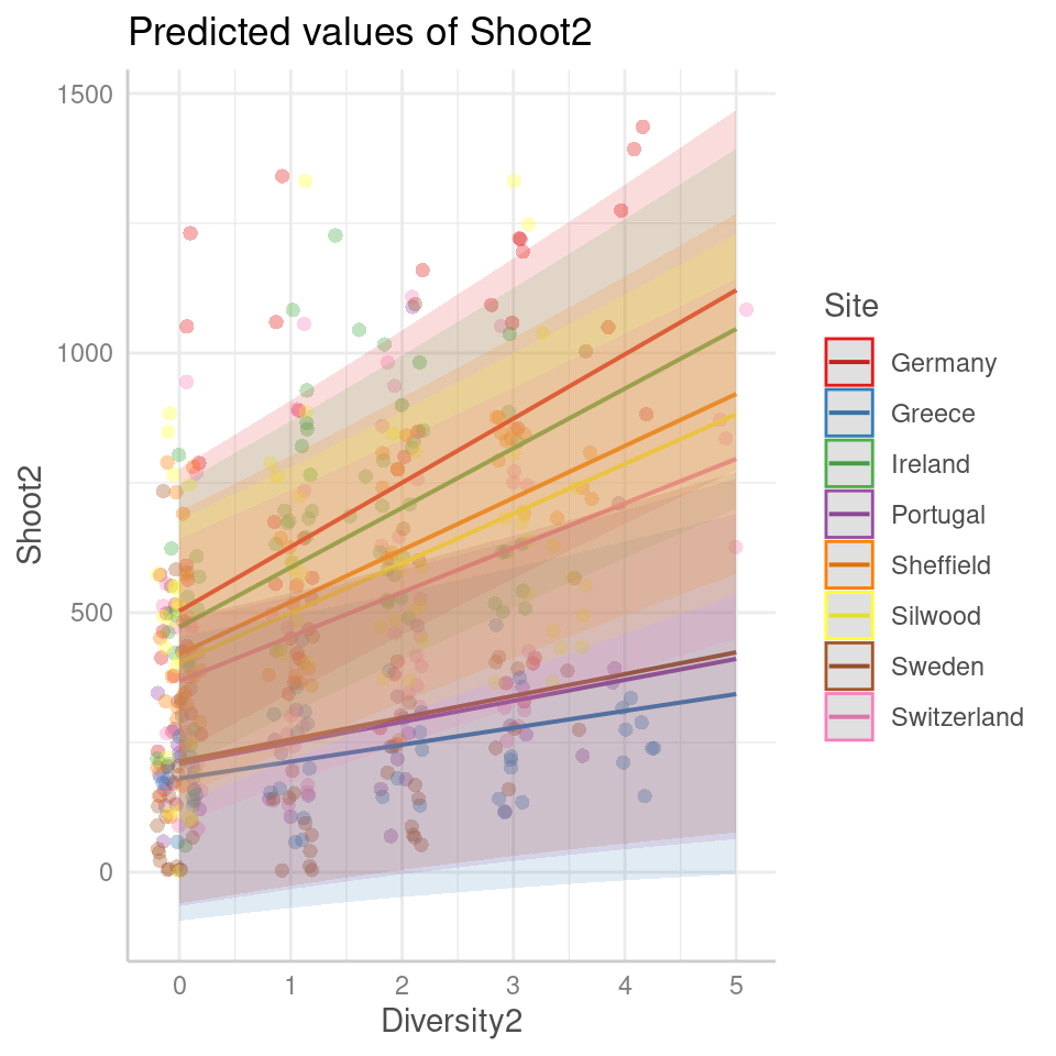
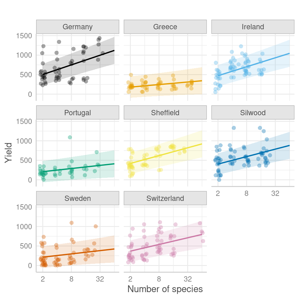
We have covered some of the packages that allow us to easily produce marginal and conditional fits, along with 95% confidence or prediction intervals: these will output ggplot2 figures, allowing plenty of customisation for presentation

ggpredict(bio.lmer2, terms = c("Diversity2", "Site"), type = "random") %>% 
plot(., add.data = TRUE)

# Custom colors
custom.col <- c("#000000", "#E69F00", "#56B4E9", "#009E73",
                "#F0E442", "#0072B2", "#D55E00", "#CC79A7")

# Create the plot with ggpredict and customization
ggpredict(bio.lmer2, terms = c("Diversity2", "Site"), type = "random") %>% 
  plot(., add.data = TRUE) + 
  facet_wrap(~ group) +
  theme(legend.position = "none") +
  scale_colour_manual(values = custom.col) +  # Custom line colors
  scale_fill_manual(values = custom.col) +  # Custom fill colors
  labs(y = "Yield", 
       x = "Number of species",
       title = "") +  # Axis and title labels
  scale_x_continuous(breaks = c(0, 2, 4), 
                     labels = c("2", "8", "32"))  # Specify x-axis breaks and labels

Scatter plot of predicted yield as a function of the number of species for different sites and experimental groups. The plot showcases the predicted conditional fixed effects and random effects 95% prediction intervals.

Figure 7.1: Scatter plot of predicted yield as a function of the number of species for different sites and experimental groups. The plot showcases the predicted conditional fixed effects and random effects 95% prediction intervals.

# Note ggpredict codes random effects as "groups" with a hidden label

###

ggpredict(bio.lmer2, terms = c("Diversity2", "Site"), 
          type = "random") %>% tibble() %>% 
  head()

predicted	std.error	conf.low	conf.high	group
503.0749	139.4697	228.96873	777.1810	Germany
180.4816	139.4697	-93.62451	454.5877	Greece
472.1150	139.4697	198.00891	746.2212	Ireland
208.5750	139.4697	-65.53108	482.6812	Portugal
420.2317	139.4697	146.12555	694.3378	Sheffield
403.9469	139.4697	129.84073	678.0530	Silwood

7.3 Write-ups

Part of the easystats range of packages (along with performance) - report(Makowski et al. (2023)) is a phenomenally powerful package for aiding in write-up and making sure all important statistics are reported.

It should however be no substitute for logic and human understanding.

library(report)
report(bio.lmer2)

## We fitted a linear mixed model (estimated using REML and nloptwrap optimizer)
## to predict Shoot2 with Diversity2 (formula: Shoot2 ~ Diversity2). The model
## included Diversity2 as random effects (formula: list(~Diversity2 | Site, ~1 |
## Site:Mix, ~1 | Mix, ~1 | Block)). The model's total explanatory power is
## substantial (conditional R2 = 0.83) and the part related to the fixed effects
## alone (marginal R2) is of 0.11. The model's intercept, corresponding to
## Diversity2 = 0, is at 346.32 (95% CI [244.12, 448.53], t(442) = 6.66, p <
## .001). Within this model:
## 
##   - The effect of Diversity2 is statistically significant and positive (beta =
## 79.36, 95% CI [44.77, 113.94], t(442) = 4.51, p < .001; Std. beta = 0.35, 95%
## CI [0.19, 0.50])
## 
## Standardized parameters were obtained by fitting the model on a standardized
## version of the dataset. 95% Confidence Intervals (CIs) and p-values were
## computed using a Wald t-distribution approximation.

Note report produces the t statistic and the estimated degrees freedom from the full model for each coefficient. I might recommend using the anova() or drop1() functions and report overall variance explained by a fixed effect with an F-test, rather than reporting each individual coefficient relative to the intercept

drop1(bio.lmer2, test = "F")

	Sum Sq	Mean Sq	NumDF	DenDF	F value	Pr(>F)
Diversity2	340561.5	340561.5	1	9.288082	20.33525	0.0013567

6 Worked Example 3 - Complex Designs

8 Worked Example 4