1 Foundations of Mixed Modelling
1.1 What is a mixed model?
Mixed models (also known as linear mixed models or hierarchical linear models) are statistical tests that build on the simpler tests of regression, t-tests and ANOVA. All of these tests are special cases of the general linear model; they all fit a straight line to data to explain variance in a systematic way.
The key difference with a linear mixed-effects model is the inclusion of random effects - variables where our observations are grouped into subcategories that systematically affect our outcome - to account for important structure in our data.
The mixed-effects model can be used in many situations instead of one of our more straightforward tests when this structure may be important. The main advantages of this approach are:
- mixed-effects models account for more of the variance
- mixed-effects models incorporate group and even individual-level differences
- mixed-effects models cope well with missing data, unequal group sizes and repeated measurements
1.2 Fixed vs Random effects
Fixed effects and random effects are terms commonly used in mixed modeling, which is a statistical framework that combines both in order to analyze data.
In mixed modeling, the fixed effects are used to estimate the overall relationship between the predictors and the response variable, while the random effects account for the within-group variability and allow for the modeling of the individual differences or group-specific effects.
The hierarchical structure of data refers to a data organization where observations are nested within higher-level groups or clusters. For example, students nested within classrooms, patients nested within hospitals, or employees nested within companies. This hierarchical structure introduces dependencies or correlations within the data, as observations within the same group tend to be more similar to each other than observations in different groups.
The need for mixed models arises when we want to account for these dependencies and properly model the variability at different levels of the hierarchy. Traditional regression models, such as ordinary least squares (OLS), assume that the observations are independent of each other. However, when working with hierarchical data, this assumption is violated, and ignoring the hierarchical structure can lead to biased or inefficient estimates, incorrect standard errors, and misleading inference.
By including random effects, mixed models allow for the estimation of both within-group and between-group variability. They provide a flexible framework for modeling the individual or group-specific effects and can capture the heterogeneity within and between groups. Additionally, mixed models can handle unbalanced or incomplete data, where some groups may have different numbers of observations.
1.2.1 Fixed effects
In broad terms, fixed effects are variables that we expect will affect the dependent/response variable: they’re what you call explanatory variables in a standard linear regression.
Fixed effects are more common than random effects, at least in their use. Fixed effects estimate different levels with no relationship assumed between the levels. For example, in a model with a dependent variable of body length and a fixed effect for fish sex, you would get an estimate of mean body length for males and then an estimate for females separately.
We can consider this in terms of a very simple linear model, here the estimated intercept is the expected value of the outcome \(y\) when the predictor \(x\) has a value of 0. The estimated slope is the expected change in \(y\) for a single unit change in \(x\). These parameters are "fixed", meaning that each individual in the population has the same expected value for the intercept and slope.
The difference between the expected value and true value is called "residual error".
\[Y_i = \beta_0 + \beta_1X_i + \epsilon_i\]
1.2.1.1 Examples:
Medical Research: In a clinical trial studying the effectiveness of different medications for treating a specific condition, the fixed effects could include categorical variables such as treatment group (e.g., medication A, medication B, placebo) or dosage level (e.g., low, medium, high). These fixed effects would capture the systematic differences in the response variable (e.g., symptom improvement) due to the specific treatment received.
Education Research: Suppose a study examines the impact of teaching methods on student performance in different schools. The fixed effects in this case might include variables such as school type (e.g., public, private), curriculum approach (e.g., traditional, progressive), or classroom size. These fixed effects would help explain the differences in student achievement across schools, accounting for the systematic effects of these factors.
Environmental Science: Imagine a study investigating the factors influencing bird species richness across different habitats. The fixed effects in this context could include variables such as habitat type (e.g., forest, grassland, wetland), habitat disturbance level (e.g., low, medium, high), or geographical region. These fixed effects would capture the systematic variations in bird species richness associated with the specific habitat characteristics.
Fixed effects are the default effects that we all learn as we begin to understand statistical concepts, and fixed effects are the default effects in functions like lm() and aov().
1.2.2 Random effects
Random effects are less commonly used but perhaps more widely encountered in nature. Each level can be considered a random variable from an underlying process or distribution in a random effect.
A random effect is a parameter that is allowed to vary across groups or individuals. Random effects do not take a single fixed value, rather they follow a distribution (usually the normal distribution). Random effects can be added to a model to account for variation around an intercept or slope. Each individual or group then gets their own estimated random effect, representing an adjustment from the mean.
So random effects are usually grouping factors for which we are trying to control. They are always categorical, as you can’t force R to treat a continuous variable as a random effect. A lot of the time we are not specifically interested in their impact on the response variable, but we know that they might be influencing the patterns we see.
1.2.2.1 Examples:
Longitudinal Health Study: Consider a study tracking the blood pressure of individuals over multiple time points. In this case, a random effect can be included to account for the individual-specific variation in blood pressure. Each individual's blood pressure measurements over time would be treated as repeated measures within that individual, and the random effect would capture the variability between individuals that is not explained by the fixed effects. This random effect allows for modeling the inherent individual differences in blood pressure levels.
Social Network Analysis: Suppose a study examines the influence of peer groups on adolescent behavior. The study may collect data on individual behaviors within schools, where students are nested within classrooms. In this scenario, a random effect can be incorporated at the classroom level to account for the shared social environment within each classroom. The random effect captures the variability in behavior among classrooms that is not accounted for by the fixed effects, enabling the study to analyze the effects of individual-level and classroom-level factors simultaneously.
Ecological Study: Imagine a research project investigating the effect of environmental factors on species abundance in different study sites. The study sites may be geographically dispersed, and a random effect can be included to account for the variation between study sites. The random effect captures the unexplained heterogeneity in species abundance across different sites, allowing for the examination of the effects of environmental variables while accounting for site-specific differences.
The random effect \(U_i\) is often assumed to follow a normal distribution with a mean of zero and a variance estimated during the model fitting process.
\[Y_i = β_0 + U_j + ε_i\]
In the book “Data analysis using regression and multilevel/hierarchical models” (Gelman & Hill (2006)). The authors examined five definitions of fixed and random effects and found no consistent agreement.
-
Fixed effects are constant across individuals, and random effects vary. For example, in a growth study, a model with random intercepts a_i and fixed slope b corresponds to parallel lines for different individuals i, or the model y_it = a_i + b t thus distinguish between fixed and random coefficients.
-
Effects are fixed if they are interesting in themselves or random if there is interest in the underlying population.
-
“When a sample exhausts the population, the corresponding variable is fixed; when the sample is a small (i.e., negligible) part of the population the corresponding variable is random.”
-
“If an effect is assumed to be a realized value of a random variable, it is called a random effect.”
-
Fixed effects are estimated using least squares (or, more generally, maximum likelihood) and random effects are estimated with shrinkage.
Thus it turns out fixed and random effects are not born but made. We must make the decision to treat a variable as fixed or random in a particular analysis.
When determining what should be a fixed or random effect in your study, consider what are you trying to do? What are you trying to make predictions about? What is just variation (a.k.a “noise”) that you need to control for?
More about random effects:
Note that the golden rule is that you generally want your random effect to have at least five levels. So, for instance, if we wanted to control for the effects of fish sex on body length, we would fit sex (a two level factor: male or female) as a fixed, not random, effect.
This is, put simply, because estimating variance on few data points is very imprecise. Mathematically you could, but you wouldn’t have a lot of confidence in it. If you only have two or three levels, the model will struggle to partition the variance - it will give you an output, but not necessarily one you can trust.
Finally, keep in mind that the name random doesn’t have much to do with mathematical randomness. Yes, it’s confusing. Just think about them as the grouping variables for now. Strictly speaking it’s all about making our models representative of our questions and getting better estimates. Hopefully, our next few examples will help you make sense of how and why they’re used.
There’s no firm rule as to what the minimum number of factor levels should be for random effect and really you can use any factor that has two or more levels. However it is commonly reported that you may want five or more factor levels for a random effect in order to really benefit from what the random effect can do (though some argue for even more, 10 levels). Another case in which you may not want to random effect is when you don’t want your factor levels to inform each other or you don’t assume that your factor levels come from a common distribution. As noted above, male and female is not only a factor with only two levels but oftentimes we want male and female information estimated separately and we’re not necessarily assuming that males and females come from a population of sexes in which there is an infinite number and we’re interested in an average.
1.3 Why use mixed models?
The provided code generates a dataset that is suitable for testing mixed models. Let's break down the code and annotate each step:
# Generating a fake dataset with different means for each group
set.seed(123)  # Setting seed for reproducibility


rand_eff <- data.frame(group = as.factor(seq(1:5)),
            b0 = rnorm(5, mean = 0, sd = 20),
            b1 = rnorm(5, 0, 0.5))
This section creates a data frame called rand_eff containing random effects. It consists of five levels of a grouping variable (group), and for each level, it generates random effects (b0 and b1) using the rnorm function.
data <- expand.grid(group = as.factor(seq(1:10)),
                    obs = as.factor(seq(1:100))) %>%
  left_join(rand_eff,
            by = "group") %>%
  mutate(x = runif(n = nrow(.), 0, 10),
         B0 = 20,
         B1 = 2,
         E = rnorm(n = nrow(.), 0, 10)) %>%
  mutate(y = B0 + b0 + x * (B1 + b1) + E)

data <- expand.grid(group = as.factor(seq(1:4)),
                    obs = as.factor(seq(1:100)))
This section creates the main dataset (data) for testing mixed models. It uses expand.grid to create a combination of levels for the grouping variable (group) and observation variable (obs). It then performs a left join with the rand_eff data frame, matching the group variable to incorporate the random effects for each group.
The code continues to mutate the dataset by adding additional variables:
x is a random predictor variable generated using
runifto have values between 0 and 10.B0 and B1 represent fixed effects of the intercept and slope with predetermined values of 20 and 2, respectively.
E represents the error term, generated using
rnormwith a mean of 0 and standard deviation of 10.Finally, y is created as the response variable using a linear model equation that includes the fixed effects (B0 and B1), random effects (b0 and b1), the predictor variable (x), and the error term (E).
data.1 <- expand.grid(group = as.factor(5),
          obs = as.factor(seq(1:30)))

data <- bind_rows(data, data.1) %>%
  left_join(rand_eff,
            by = "group") %>%
  mutate(x = runif(n = nrow(.), 0, 10),
         B0 = 20,
         B1 = 2,
         E = rnorm(n = nrow(.), 0, 10)) %>%
  mutate(y = B0 + b0 + x * (B1 + b1) + E)
This section creates an additional dataset (data.1) with a specific group (group = 5) and a smaller number of observations (obs = 30) for testing purposes. This is then appended to the original dataset, we will see the effect of having a smaller group within our random effects when we discuss partial pooling and shrinkage later on.
Now we have three variables to consider in our models: x, y and group (with five levels).
| x | y | group | obs |
|---|---|---|---|
| 4.0584411 | -0.5487802 | 1 | 1 |
| 7.2250893 | 17.3260398 | 2 | 1 |
| 0.5963383 | 41.2256737 | 3 | 1 |
| 3.3034922 | 16.0958571 | 4 | 1 |
| 7.7676400 | 32.0586590 | 1 | 2 |
| 8.4045935 | 50.1274193 | 2 | 2 |
Now that we have a suitable simulated dataset, let's start modelling!
1.3.1 All in one model
We will begin by highlighting the importance of considering data structure and hierarchy when building linear models. To illustrate this, we will delve into an example that showcases the consequences of ignoring the underlying data structure. We might naively construct a single linear model that ignores the group-level variation and treats all observations as independent. This oversimplified approach fails to account for the fact that observations within groups are more similar to each other due to shared characteristics.
\[Y_i = \beta_0 + \beta_1X_i + \epsilon_i\]
##
## Call:
## lm(formula = y ~ x, data = data)
##
## Residuals:
##    Min     1Q Median     3Q    Max
## -37.23 -12.11  -2.36  11.00  44.53
##
## Coefficients:
##             Estimate Std. Error t value Pr(>|t|)
## (Intercept)  21.0546     1.6490  12.768   <2e-16 ***
## x             2.5782     0.2854   9.034   <2e-16 ***
## ---
## Signif. codes:  0 '***' 0.001 '**' 0.01 '*' 0.05 '.' 0.1 ' ' 1
##
## Residual standard error: 16.96 on 428 degrees of freedom
## Multiple R-squared:  0.1602, Adjusted R-squared:  0.1582
## F-statistic: 81.62 on 1 and 428 DF,  p-value: < 2.2e-16
Here we can see that the basic linear model has produced a statistically significant regression analysis (t428 = 9.034, p <0.001) with an \(R^2\) of 0.16. There is a medium effect positive relationship between changes in x and y (Estimate = 2.58, S.E. = 0.29).
We can see that clearly if we produce a simple plot of x against y:
plot(data$x, data$y)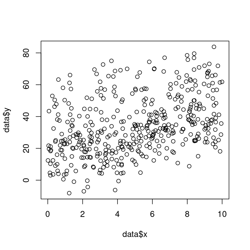
Figure 1.1: Simple scatter plot x against y
Here if we use the function geom_smooth() on the scatter plot, the plot also includes a fitted regression line obtained using the "lm" method. This allows us to examine the overall trend and potential linear association between the variables.
ggplot(data, aes(x = x,
                 y = y)) +
  geom_point() +
  labs(x = "Independent Variable",
       y = "Dependent Variable")+
  geom_smooth(method = "lm")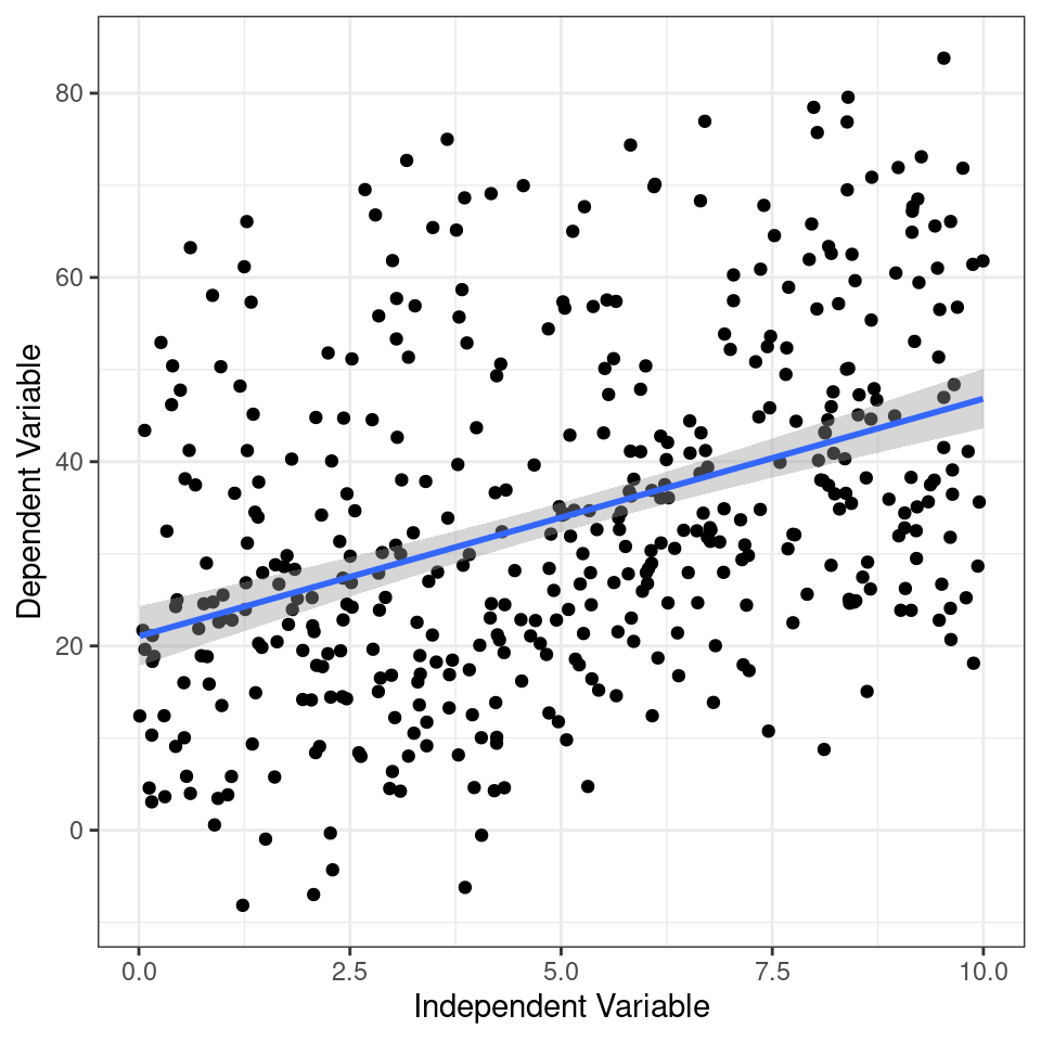
Figure 1.2: Scatter plot displaying the relationship between the independent variable and the dependent variable. The points represent the observed data, while the fitted regression line represents the linear relationship between the variables. The plot helps visualize the trend and potential association between the variables.
The check_model() function from the performance package (Lüdecke et al. (2023)) is used to evaluate the performance and diagnostic measures of a statistical model. It provides a comprehensive assessment of the model's fit, assumptions, and predictive capabilities. By calling this function, you can obtain a summary of various evaluation metrics and diagnostic plots for the specified model.
It enables you to identify potential issues, such as violations of assumptions, influential data points, or lack of fit, which can affect the interpretation and reliability of your model's results
performance::check_model(basic_model)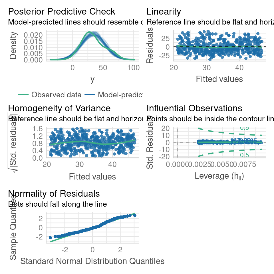
Looking at the fit of our model we would be tempted to conclude that we have an accurate and robust model.
However, when data is hierarchically structured, such as individuals nested within groups, there is typically correlation or similarity among observations within the same group. By not accounting for this clustering effect, estimates derived from a single model can be biased and inefficient. The assumption of independence among observations is violated, leading to incorrect standard errors and inflated significance levels.
From the figure below we can see the difference in median and range of x values within each of our groups:
ggplot(data, aes(x = group,
                 y = y)) +
  geom_boxplot() +
  labs(x = "Groups",
       y = "Dependent Variable")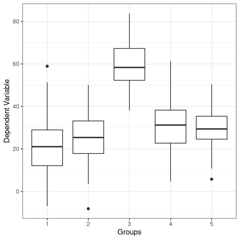
Figure 1.3: Linear model conducted on all data
In this figure, we colour tag the data points by group, this can be useful for determining if a mixed model is appropriate.
Here's why:
By colour-coding the data points based on the grouping variable, the plot allows you to visually assess the within-group and between-group variability. If there are noticeable differences in the data patterns or dispersion among the groups, it suggests that the data may have a hierarchical structure, where observations within the same group are more similar to each other than to observations in other groups.
# Color tagged by group
plot_group <- ggplot(data, aes(x = x,
                               y = y,
                               color = group,
                               group = group)) +
  geom_point(alpha = 0.6) +
  labs(title = "Data Coloured by Group",
       x = "Independent Variable",
       y = "Dependent Variable")+
  theme(legend.position="none")

plot_group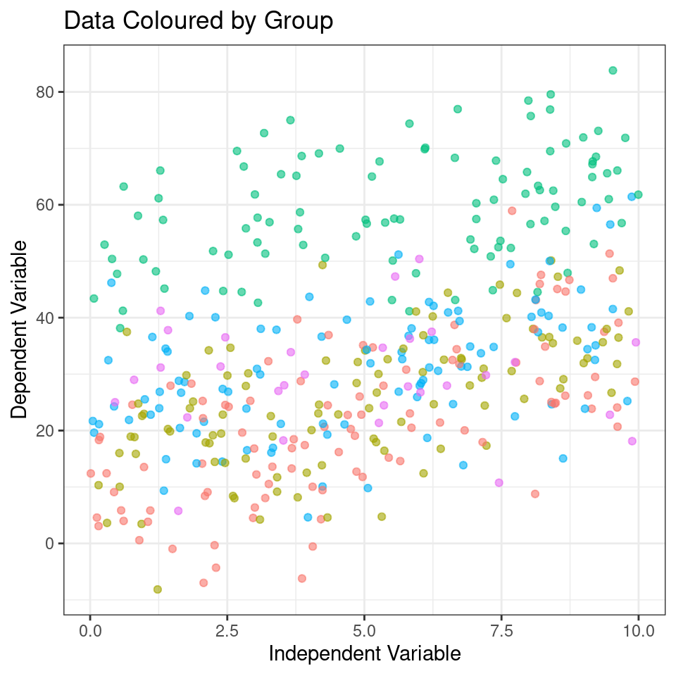
From the above plots, it confirms that our observations from within each of the ranges aren’t independent. We can’t ignore that: as we’re starting to see, it could lead to a completely erroneous conclusion.
1.3.2 Multiple analyses approach
Running separate linear models per group, also known as stratified analysis, can be a feasible approach in certain situations. However, there are several drawbacks including
Increased complexity
Inability to draw direct conclusions on overall variability
Reduced statistical power
Inflated Type 1 error risk
Inconsistent estimates
Limited ability to handle unbalanced/missing data
# Plotting the relationship between x and y with group-level smoothing
ggplot(data, aes(x = x, y = y, color = group, group = group)) +
  geom_point(alpha = 0.6) +  # Scatter plot of x and y with transparency
  labs(title = "Data Colored by Group", x = "Independent Variable", y = "Dependent Variable") +
  theme(legend.position = "none") +
  geom_smooth(method = "lm") +  # Group-level linear regression smoothing
  facet_wrap(~group)  # Faceting the plot by group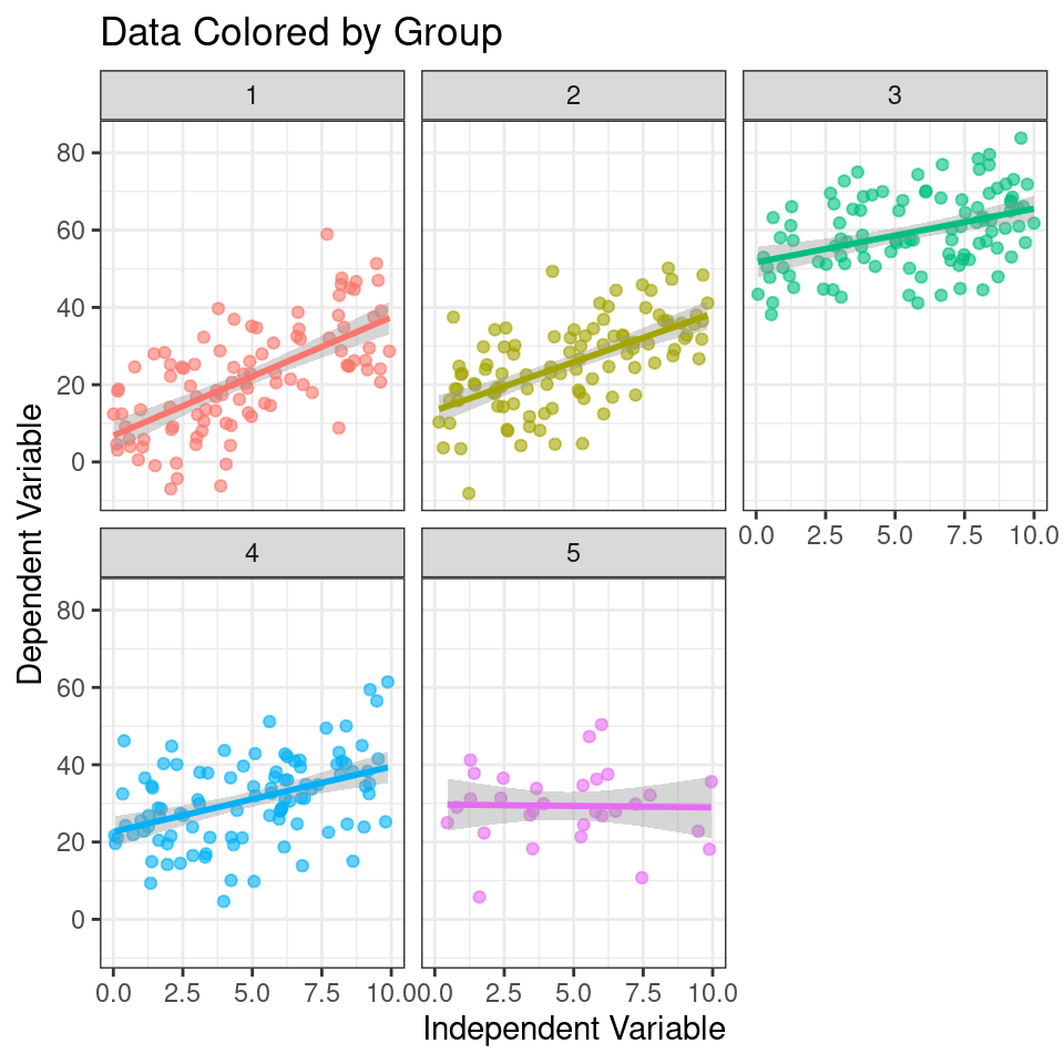
Figure 1.4: Scatter plot showing the relationship between the independent variable (x) and the dependent variable (y) colored by group. Each subplot represents a different group. The line represents the group-level linear regression smoothing.
# Creating nested data by grouping the data by 'group'
nested_data <- data %>%
  group_by(group) %>%
  nest()

# Fitting linear regression models to each nested data group
models <- map(nested_data$data, ~ lm(y ~ x, data = .)) %>%
          map(broom::tidy)

# Combining the model results into a single data frame
combined_models <- bind_rows(models)

# Filtering the rows to include only the 'x' predictor
filtered_models <- combined_models %>%
                   filter(term == "x")

# Adding a column for the group index using rowid_to_column function
group_indexed_models <- filtered_models %>%
                        rowid_to_column("group")

# Modifying the p-values using a custom function report_p
final_models <- group_indexed_models %>%
                mutate(p.value = report_p(p.value))

final_models| group | term | estimate | std.error | statistic | p.value |
|---|---|---|---|---|---|
| 1 | x | 3.0643940 | 0.3620254 | 8.4645823 | p < 0.001 |
| 2 | x | 2.5162898 | 0.3354848 | 7.5004590 | p < 0.001 |
| 3 | x | 1.3904720 | 0.3192878 | 4.3549169 | p < 0.001 |
| 4 | x | 1.6856649 | 0.3550511 | 4.7476686 | p < 0.001 |
| 5 | x | -0.0755633 | 0.6576868 | -0.1148926 | p= 0.909 |
In the code above, the dataset data is first grouped by the variable 'group' using the group_by function, and then the data within each group is nested using the nest function. This results in a new dataset nested_data where each group's data is stored as a nested tibble.
Next, a linear regression model (lm) is fit to each nested data group using the map function. The broom::tidy function is applied to each model using map to extract the model summary statistics, such as coefficients, p-values, and standard errors. The resulting models are stored in the models object.
The bind_rows function is used to combine the model results into a single data frame called combined_models. The data frame is then filtered to include only the rows where the predictor is 'x' using the filter function, resulting in the filtered_models data frame.
To add a column for the group index, the rowid_to_column function is applied to the filtered_models data frame, creating the group_indexed_models data frame with an additional column named 'group'.
Finally, the p-values in the group_indexed_models data frame are modified using a custom function report_p
1.3.3 Complex model
Using a group level term with an interaction on x as a fixed effect means explicitly including the interaction term between x and the group as a predictor in the model equation. This approach assumes that the relationship between x and the outcome variable differs across groups and that these differences are constant and fixed. It implies that each group has a unique intercept (baseline level) and slope (effect size) for the relationship between x and the outcome variable. By treating the group level term as a fixed effect, the model estimates specific parameter values for each group.
If we are not explicitly interested in the outcomes or differences for each individual group (but wish to account for them) - this may not be the best option as it can lead to overfitting and it uses a lot more degrees of freedom - impacting estimates and widening our confidence intervals. As with running multiple models above, there is limited ability to make inferences outside of observed groups, and it does not handle missing data or unbalanced designs well.
\[Y_i = \beta_0 + \beta_1X_i + \beta_2.group_i+\beta_3(X_i.group_i)+\epsilon_i\]
##
## Call:
## lm(formula = y ~ x * group, data = data)
##
## Residuals:
##      Min       1Q   Median       3Q      Max
## -24.8614  -6.2579   0.2044   6.9342  28.5474
##
## Coefficients:
##             Estimate Std. Error t value Pr(>|t|)
## (Intercept)   6.8125     1.8881   3.608 0.000346 ***
## x             3.0644     0.3379   9.070  < 2e-16 ***
## group2        6.4526     2.7289   2.365 0.018505 *
## group3       44.8356     2.8539  15.710  < 2e-16 ***
## group4       15.8607     2.7184   5.835 1.08e-08 ***
## group5       22.9090     4.0772   5.619 3.51e-08 ***
## x:group2     -0.5481     0.4875  -1.124 0.261560
## x:group3     -1.6739     0.4781  -3.501 0.000513 ***
## x:group4     -1.3787     0.4830  -2.855 0.004522 **
## x:group5     -3.1400     0.7479  -4.198 3.28e-05 ***
## ---
## Signif. codes:  0 '***' 0.001 '**' 0.01 '*' 0.05 '.' 0.1 ' ' 1
##
## Residual standard error: 9.801 on 420 degrees of freedom
## Multiple R-squared:  0.7246, Adjusted R-squared:  0.7187
## F-statistic: 122.8 on 9 and 420 DF,  p-value: < 2.2e-16
1.4 Our first mixed model
A mixed model is a good choice here: it will allow us to use all the data we have (higher sample size) and account for the correlations between data coming from the groups. We will also estimate fewer parameters and avoid problems with multiple comparisons that we would encounter while using separate regressions.
We can now join our random effect \(U_j\) to the full dataset and define our y values as
\[Y_{ij} = β_0 + β_1*X_{ij} + U_j + ε_{ij}\].
We have a response variable, and we are attempting to explain part of the variation in test score through fitting an independent variable as a fixed effect. But the response variable has some residual variation (i.e. unexplained variation) associated with group. By using random effects, we are modeling that unexplained variation through variance.
We now want to know if an association between y ~ x exists after controlling for the variation in group.
1.4.1 Running mixed effects models with lmerTest
This section will detail how to run mixed models with the lmer function in the R package lmerTest (Kuznetsova et al. (2020)). This builds on the older lme4 (Bates et al. (2023)) package, and in particular add p-values that were not previously included. There are other R packages that can be used to run mixed-effects models including the nlme package (Pinheiro et al. (2023)) and the glmmTMB package (Brooks et al. (2023)). Outside of R there are also other packages and software capable of running mixed-effects models, though arguably none is better supported than R software.
plot_function2 <- function(model, title = "Data Coloured by Group"){

data <- data %>%
  mutate(fit.m = predict(model, re.form = NA),
         fit.c = predict(model, re.form = NULL))

data %>%
  ggplot(aes(x = x, y = y, col = group)) +
  geom_point(pch = 16, alpha = 0.6) +
  geom_line(aes(y = fit.c, col = group), linewidth = 2)  +
  coord_cartesian(ylim = c(-40, 100))+
  labs(title = title,
       x = "Independent Variable",
       y = "Dependent Variable")
}

mixed_model <- lmer(y ~ x + (1|group), data = data)

plot_function2(mixed_model, "Random intercept")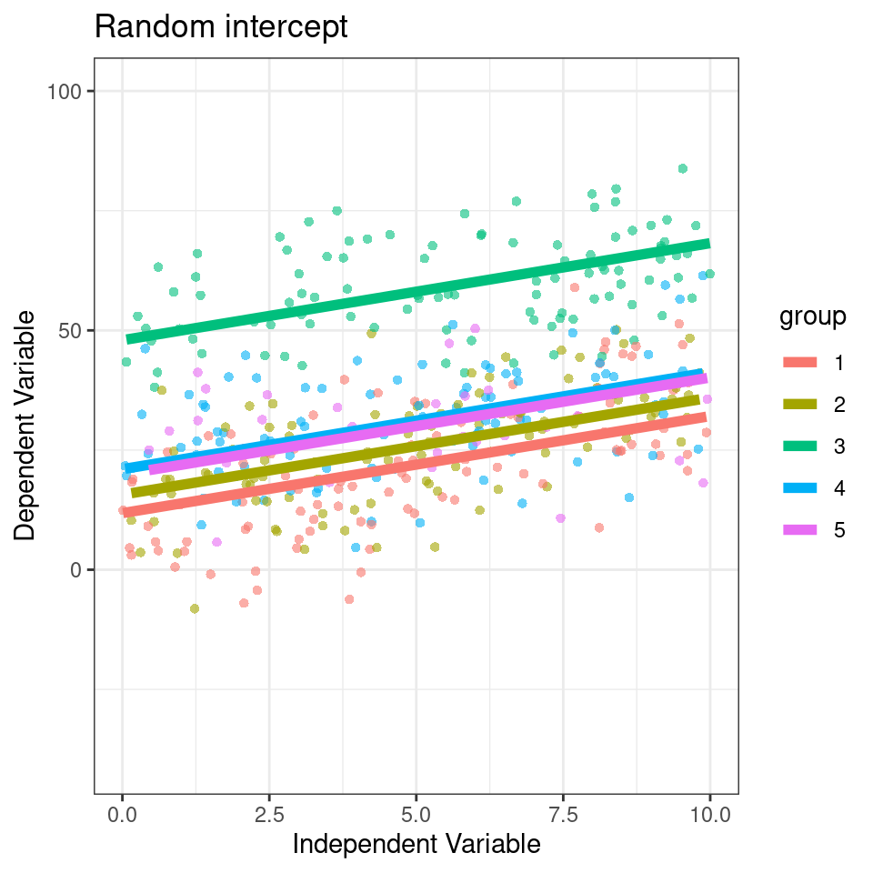
## Linear mixed model fit by REML. t-tests use Satterthwaite's method [
## lmerModLmerTest]
## Formula: y ~ x + (1 | group)
##    Data: data
##
## REML criterion at convergence: 3224.4
##
## Scaled residuals:
##      Min       1Q   Median       3Q      Max
## -2.61968 -0.63654 -0.03584  0.66113  3.13597
##
## Random effects:
##  Groups   Name        Variance Std.Dev.
##  group    (Intercept) 205      14.32
##  Residual             101      10.05
## Number of obs: 430, groups:  group, 5
##
## Fixed effects:
##             Estimate Std. Error       df t value Pr(>|t|)
## (Intercept)  23.2692     6.4818   4.1570    3.59   0.0215 *
## x             2.0271     0.1703 424.0815   11.90   <2e-16 ***
## ---
## Signif. codes:  0 '***' 0.001 '**' 0.01 '*' 0.05 '.' 0.1 ' ' 1
##
## Correlation of Fixed Effects:
##   (Intr)
## x -0.131
Here our groups clearly explain a lot of variance
205/(205 + 101) = 0.669 / 66.9%
So the differences between groups explain ~67% of the variance that’s “left over” after the variance explained by our fixed effects.
1.4.2 Partial pooling
It is worth noting that random effect estimates are a function of the group-level information and the overall (grand) mean of the random effect. Group levels with low sample size or poor information (i.e., no strong relationship) are more strongly influenced by the grand mean, which adds information to an otherwise poorly-estimated group. However, a group with a large sample size or strong information (i.e., a strong relationship) will have very little influence from the grand mean and largely reflect the information contained entirely within the group. This process is called partial pooling (as opposed to no pooling, where no effect is considered, or total pooling, where separate models are run for the different groups). Partial pooling results in the phenomenon known as shrinkage, which refers to the group-level estimates being shrunk toward the mean. What does all this mean? If you use a random effect, you should be prepared for your factor levels to have some influence from the overall mean of all levels. With a good, clear signal in each group, you won’t see much impact from the overall mean, but you will with small groups or those without much signal.
Below we can take a look at the estimates and standard errors for three of our previously constructed models:
pooled <- basic_model %>%
  broom::tidy() %>%
  mutate(Approach = "Pooled", .before = 1) %>%
  select(term, estimate, std.error, Approach)

no_pool <- additive_model %>%
  broom::tidy() %>%
  mutate(Approach = "No Pooling", .before = 1) %>%
  select(term, estimate, std.error, Approach)

partial_pool <- mixed_model %>%
  broom.mixed::tidy() %>%
  mutate(Approach = "Mixed Model/Partial Pool", .before = 1) %>%
  select(Approach, term, estimate, std.error)

bind_rows(pooled, no_pool, partial_pool) %>%
filter(term %in% c("x" , "(Intercept)") )| term | estimate | std.error | Approach |
|---|---|---|---|
| (Intercept) | 21.054614 | 1.6490185 | Pooled |
| x | 2.578217 | 0.2853798 | Pooled |
| (Intercept) | 6.812481 | 1.8881155 | No Pooling |
| x | 3.064394 | 0.3378685 | No Pooling |
| (Intercept) | 23.269187 | 6.4818211 | Mixed Model/Partial Pool |
| x | 2.027065 | 0.1703423 | Mixed Model/Partial Pool |
Pooling helps to improve the precision of the estimates by borrowing strength from the entire dataset. However, this can also lead to differences in the estimates and standard errors compared to models without pooling.
Pooled: in the pooled model the averaged estimates may not accurately reflect the true values within each group. As a result, the estimates in pooled models can be biased towards the average behavior across all groups. We can see this in the too small standard error of the intercept, underestimating the variance in our dataset. At the same time if there is substantial variability in the relationships between groups, the pooled estimates can be less precise. This increased variability across groups can contribute to larger standard errors of the difference (SED) for fixed effects in pooled models.
No pooling: This model is extremely precise with the smallest errors, however these estimates reflect conditions only for the first group in the model
Partial pooling/Mixed models: this model reflects the greater uncertainty of the Mean and SE of the intercept. However, the SED in a partial pooling model accounts for both the variability within groups and the uncertainty between groups. Compared to a no pooling approach, the SED in a partial pooling model tends to be smaller because it incorporates the pooled information, which reduces the overall uncertainty. This adjusted SED provides a more accurate measure of the uncertainty associated with the estimated differences between groups or fixed effects.
1.5 Predictions
One misconception about mixed-effects models is that we cannot produce estimates of the relationships for each group.
But how do we do this?
We can use the coef() function to extract the estimates (strictly these are predictions) for the random effects. This output has several components.
coef(mixed_model)## $group
## (Intercept) x
## 1 11.82356 2.027066
## 2 15.68146 2.027066
## 3 47.94678 2.027066
## 4 21.01028 2.027066
## 5 19.88385 2.027066
##
## attr(,"class")
## [1] "coef.mer"This function produces our 'best linear unbiased predictions' (BLUPs) for the intercept and slope of the regression at each site. The predictions given here are different to those we would get if we ran individual models on each site, as BLUPs are a product of the compromise of complete-pooling and no-pooling models. Now the predicted intercept is influenced by other sites leading to a process called 'shrinkage'.
Why are these called predictions and not estimates? Because we have estimated the variance at each site and from here essentially borrowed information across sites to improve the accuracy, to combine with the fixed effects. So in the strictest sense we are predicting relationships rather than through direct observation.
This generous ability to make predictions is one of the main advantages of a mixed-model.
The summary() function has already provided the estimates of the fixed effects, but they can also be extracted with the fixef() function.
fixef(mixed_model)## (Intercept) x
## 23.269187 2.027066We can also apply anova() to a single model to get an F-test for the fixed effect
anova(mixed_model)| Sum Sq | Mean Sq | NumDF | DenDF | F value | Pr(>F) | |
|---|---|---|---|---|---|---|
| x | 14303.23 | 14303.23 | 1 | 424.0815 | 141.6089 | 0 |
1.5.1 Shrinkage in mixed models
The graph below demonstrates the compromise between complete pooling and no pooling. It plots the overall regression line/mean (the fixed effects from the lmer model), the predicted slopes at each site from the mixed-effects model, and compares this to the estimates from each site (nested lm).
As you can see most of the groups show shrinkage, that is they deviate less from the overall mean, most obviously in group 5, where the sample size is deliberately reduced. Here you can see the predicted line is much closer to the overall regression line, reflecting the greater uncertainty. The slope is drawn towards the overall mean by shrinkage.
# Nesting the data by group
nested_data <- data %>%
    group_by(group) %>%
    nest()

# Fitting linear regression models and obtaining predictions for each group
nested_models <- map(nested_data$data, ~ lm(y ~ x, data = .)) %>%
    map(predict)
# Creating a new dataframe and adding predictions from different models
data1 <- data %>%
  mutate(fit.m = predict(mixed_model, re.form = NA),
         fit.c = predict(mixed_model, re.form = NULL)) %>%
  arrange(group,obs) %>%
  mutate(fit.l = unlist(nested_models))

# Creating a plot to visualize the predictions
data1 %>%
  ggplot(aes(x = x, y = y, colour = group)) +
    geom_point(pch = 16) +
  geom_line(aes(y = fit.l, linetype = "lm"), colour = "black")+
  geom_line(aes(y = fit.c, linetype = "lmer"))+
  geom_line(aes(y = fit.m, linetype = "Mean"), colour = "grey")+
   scale_linetype_manual(name = "Model Type",
                        labels = c("Mean", "lmer", "lm"),
                        values = c("dotdash", "solid", "dashed"))+
  facet_wrap( ~ group)+
  guides(colour = "none")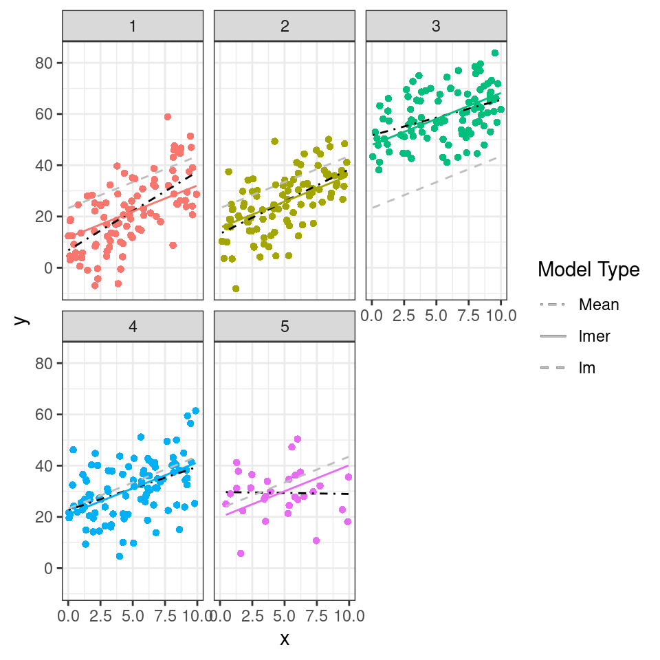
Figure 1.5: Regression relationships from fixed-effects and mixed effects models, note shrinkage in group 5
re.form = NA: When re.form is set to NA, it indicates that the random effects should be ignored during prediction. This means that the prediction will be based solely on the fixed effects of the model, ignoring the variation introduced by the random effects. This is useful when you are interested in estimating the overall trend or relationship described by the fixed effects, without considering the specific random effects of individual groups or levels.
re.form = NULL: Conversely, when re.form is set to NULL, it indicates that the random effects should be included in the prediction. This means that the prediction will take into account both the fixed effects and the random effects associated with the levels of the random effect variable. The model will use the estimated random effects to generate predictions that account for the variation introduced by the random effects. This is useful when you want to visualize and analyze the variation in the response variable explained by different levels of the random effect.
It's not always easy/straightforward to make prediciton or confidence intervals from complex general and generalized linear mixed models, luckily there are some excellent R packages that will do this for us.
1.5.2 ggeffects
ggeffects (Lüdecke (2023a)) is a light-weight package that aims at easily calculating marginal effects and adjusted predictions
1.5.2.1 ggpredict
The argument type = random in the ggpredict function (from the ggeffects package Lüdecke (2023a)) is used to specify the type of predictions to be generated in the context of mixed effects models. The main difference between using ggpredict with and without type = random lies in the type of predictions produced:
Without type = random: ggpredict will generate fixed-effects predictions. These estimates are based solely on the fixed effects of the model, ignoring any variability associated with the random effects. The resulting estimate represent the average or expected values of the response variable for specific combinations of predictor values, considering only the fixed components of the model.
Estimated mean fixed effects provide a comprehensive view of the average effect of dependent variables on the response variable. By plotting the estimated mean fixed effects using ggpredict, you can visualize how the response variable changes across different levels or values of the predictors while considering the effects of other variables in the model.
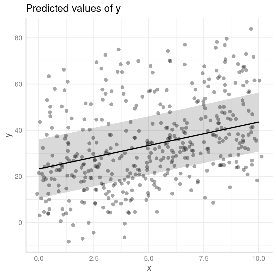
With type = random: ggpredict will generate predictions that incorporate both fixed and random effects. These predictions take into account the variability introduced by the random effects in the model. The resulting predictions reflect not only the average trend captured by the fixed effects but also the additional variability associated with the random effects at different levels of the grouping factor(s).
By default the figure now produces prediciton intervals
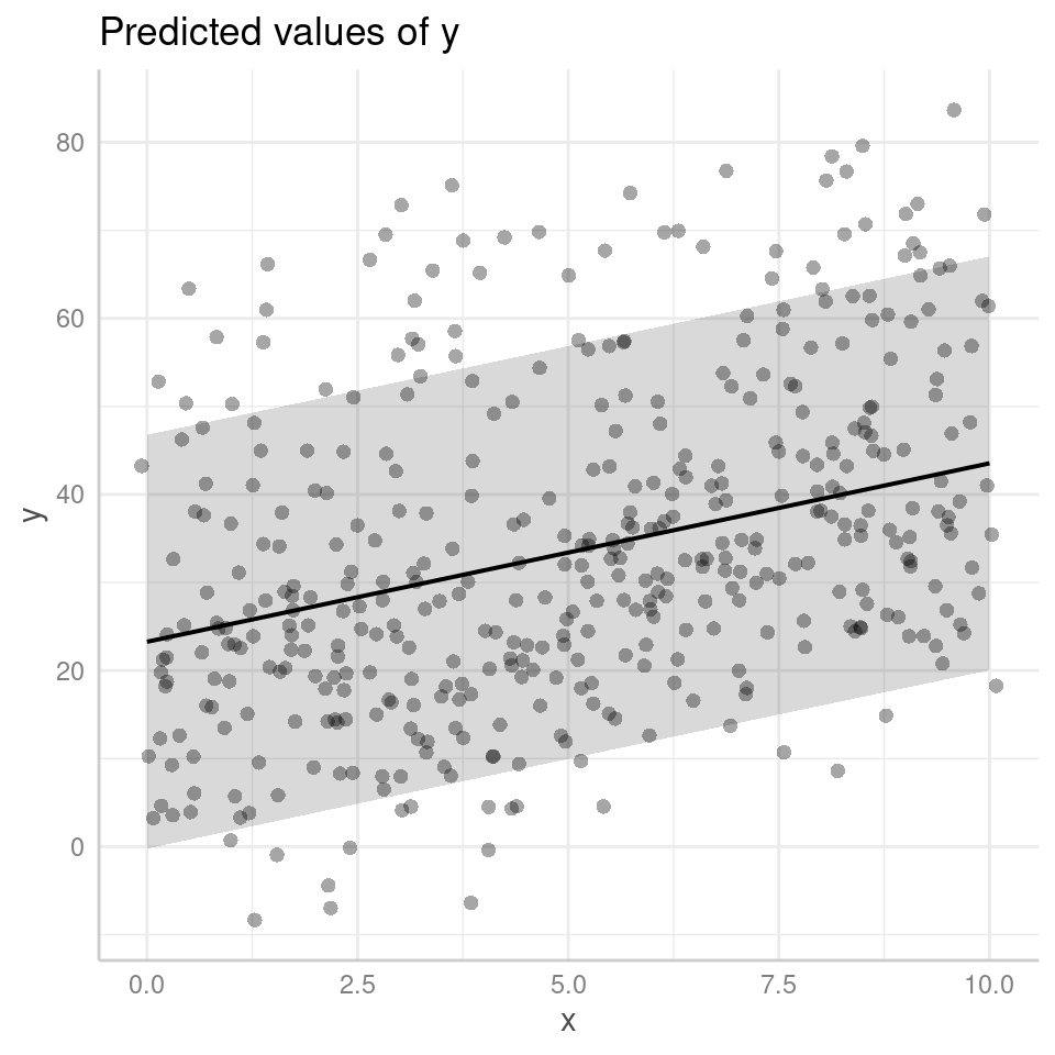
Confidence Intervals: A confidence interval is used to estimate the range of plausible values for a population parameter, such as the mean or the regression coefficient, based on a sample from that population. It provides a range within which the true population parameter is likely to fall with a certain level of confidence. For example, a 95% confidence interval implies that if we were to repeat the sampling process many times, 95% of the resulting intervals would contain the true population parameter.
Prediction Intervals: On the other hand, a prediction interval is used to estimate the range of plausible values for an individual observation or a future observation from the population. It takes into account both the uncertainty in the estimated model parameters and the inherent variability within the data. A 95% prediction interval provides a range within which a specific observed or predicted value is likely to fall with a certain level of confidence. The wider the prediction interval, the greater the uncertainty around the specific value being predicted.
Furthermore, ggpredict() enables you to explore group-level predictions, which provide a deeper understanding of how the response variable varies across different levels of the grouping variable. By specifying the desired grouping variable in ggpredict when type = random, you can generate plots that depict the predicted values for each group separately, allowing for a comparative analysis of group-level effects.
ggpredict(mixed_model, terms = c("x", "group"), type = "random") %>%
plot(., add.data = TRUE) +
  facet_wrap(~group)+
  theme(legend.position = "none")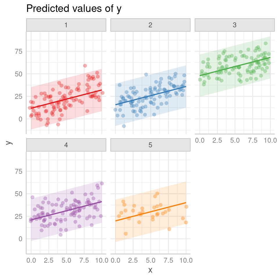
1.5.3 sjPlot
Another way to visualise mixed model results is with the package sjPlot(Lüdecke (2023b)), and if you are interested in showing the variation among levels of your random effects, you can plot the departure from the overall model estimate for intercepts - and slopes, if you have a random slope model:
library(sjPlot)

plot_model(mixed_model, terms = c("x", "group"), type = "re")/
  (plot_model(mixed_model, terms = c("x", "group"), type = "est")+ggtitle("Fixed Effects"))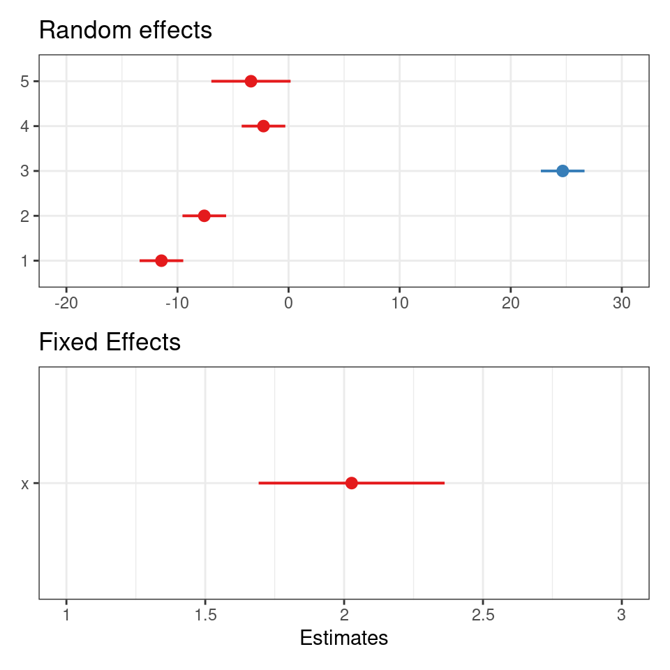
The values you see are NOT actual values, but rather the difference between the general intercept or slope value found in your model summary and the estimate for this specific level of random/fixed effect.
sjPlot is also capable of producing prediction plots in the same way as ggeffects:
plot_model(mixed_model,type="pred",
           terms=c("x", "group"),
           pred.type="re",
           show.data = T)+
  facet_wrap( ~ group)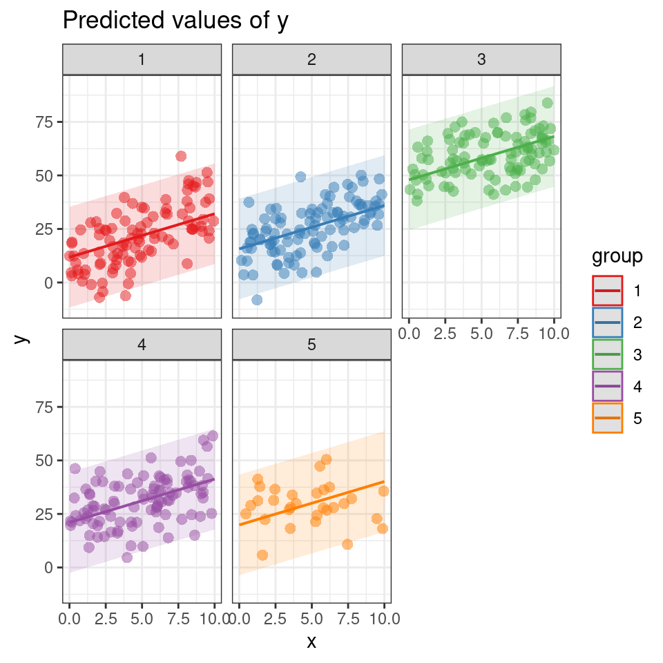
1.6 Checking model assumptions
We need to be just as conscious of testing the assumptions of mixed effects models as we are with any other. The assumptions are:
Within-group errors are independent and normally distributed with mean zero and variance \(\sigma^2\)
Within-group errors are independent of the random effects.
Random effects are normally distributed with mean zero.
Random effects are independent for different groups, except as specified by nesting (more on this later)
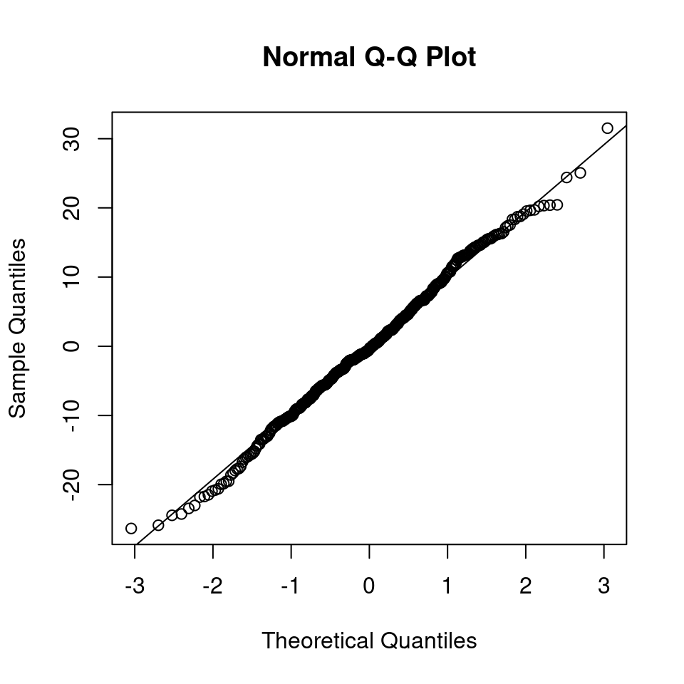
Several model check plots would help us to confirm/deny these assumptions, but note that QQ-plots may not be relevant because of the model structure. Two commonly-used plots are:
plot(mixed_model) 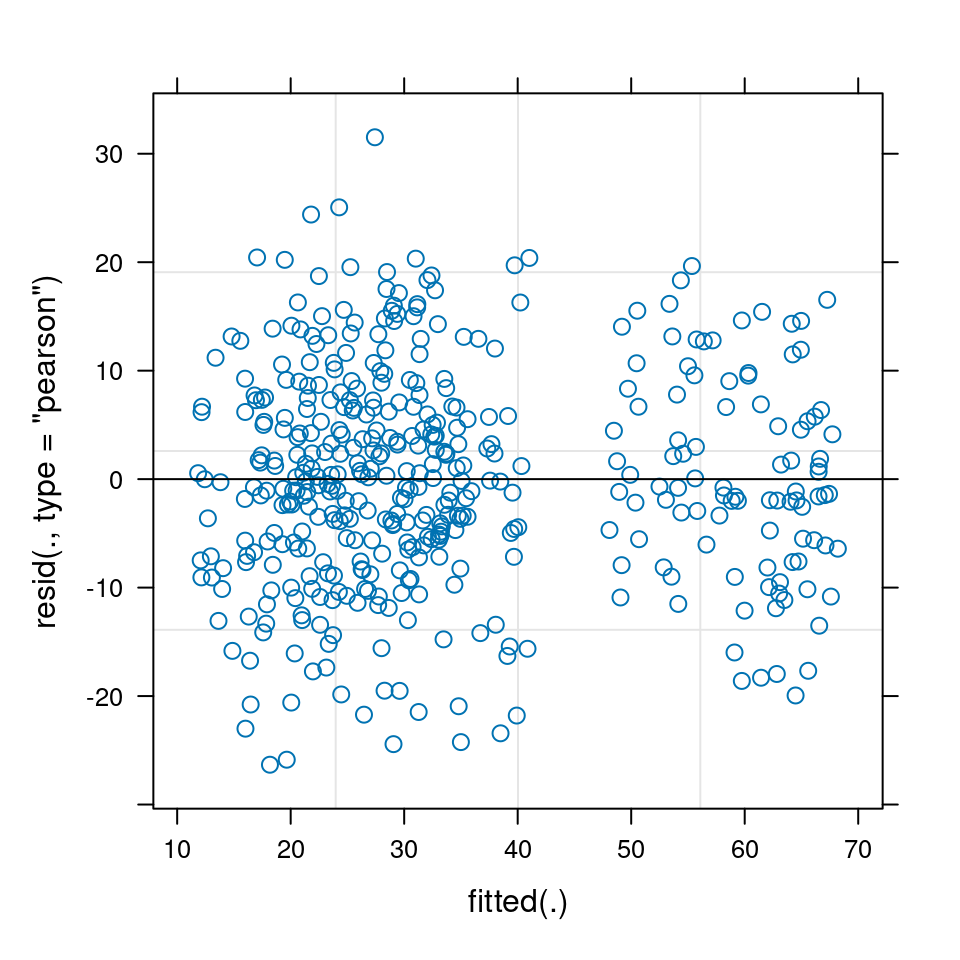
It can often be useful to check the distribution of residuals in each of the groups (e.g. blocks) to check assumptions 1 and 2. We can do this by plotting the residuals against the fitted values, separately for each level of the random effect, using the coplot() function:
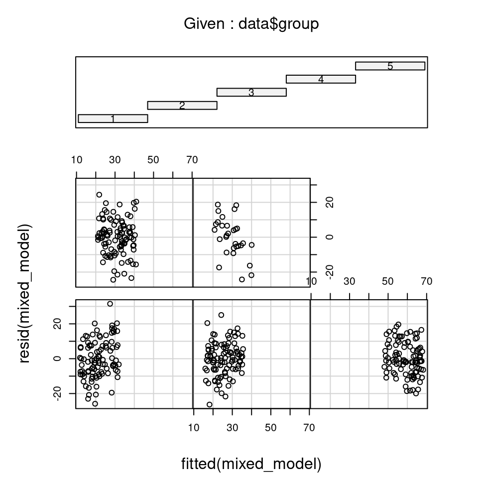
Each sub-figure of this plot, which refers to an individual group, doesn’t contain much data. It can be hard to judge whether the spread of residuals around fitted values is the same for each group when observations are low.
We can check assumption 3 with a histogram (here the more levels we have, the more we can be assured):
rand_dist <- as.data.frame(ranef(mixed_model)) %>%
  mutate(group = grp,
         b0_hat = condval,
         intercept_cond = b0_hat + summary(mixed_model)$coef[1,1],
         .keep = "none")

hist(rand_dist$b0_hat)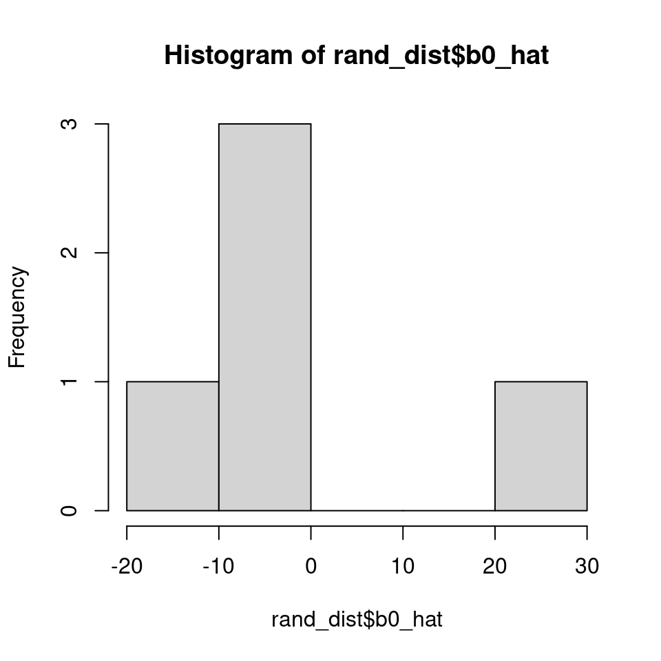
Overlaying the random distribution of our intercept over the regression line produces a plot like the below:
data1 %>%
  ggplot(aes(x = x, y = y)) +
  geom_point(pch = 16, col = "grey") +
  geom_violinhalf(data = rand_dist,
                  aes(x = 0, y = intercept_cond),
                  trim = FALSE,
                  width = 4,
                  adjust = 2,
                  fill = NA)+
  geom_line(aes(y = fit.m), linewidth = 2)  +
  coord_cartesian(ylim = c(-40, 100))+
  labs(x = "Independent Variable",
       y = "Dependent Variable")
Figure 1.6: Marginal fit, heavy black line from the random effect model with a histogram of the of the distribution of conditional intercepts
1.6.1 performance
The check_model() function from the performance package in R is a useful tool for evaluating the performance and assumptions of a statistical model, particularly in the context of mixed models. It provides a comprehensive set of diagnostics and visualizations to assess the model's fit, identify potential issues, and verify the assumptions underlying the model, which can be difficult with complex models
library(performance)
check_model(mixed_model)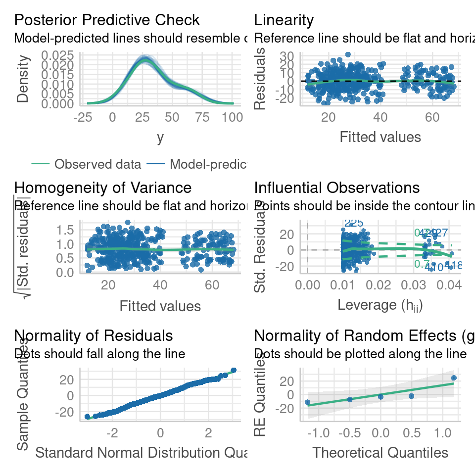
1.6.2 DHARma
Simulation-based methods, like those available with DHARMa (Hartig (2022)), are often preferred for model validation and assumption checking because they offer flexibility and do not rely on specific assumptions. Simulation is particularly useful for evaluating complex models with multiple levels of variability, non-linearity, or complex hierarchical structures. Such models may not be adequately evaluated by solely examining residuals, and simulation provides a more robust approach to assess their assumptions and performance.
Read the authors summary here
library(DHARMa)

resid.mm <- simulateResiduals(mixed_model)

plot(resid.mm)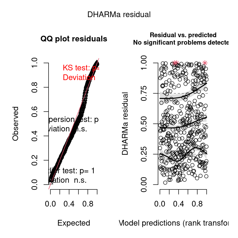
When you have a lot of data, even minimal deviations from the expected distribution will become significant (this is discussed in the help/vignette for the DHARMa package). You will need to assess the distribution and decide if it is important for yourself.